Sectioin 5. Evaluation, Boundaries, and Generalization (Some more ML Concepts)#
Understanding the Decision Boundary#
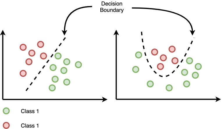
The Decision Boundary is the abstract line or surface that separates different classes in the feature space. It shows where the model switches its prediction from one class to another.
KNN and its Boundary#
For KNN, the decision boundary is inherently complex and non-linear. Its shape is directly dependent on the training data points and the value of \(k\):
The boundary exists where the majority vote of the \(k\) closest neighbors changes.
A small \(k\) results in a very jagged, flexible boundary.
A large \(k\) results in a very smooth, simple boundary.
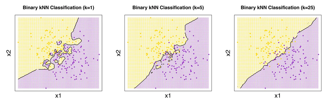
For example, here for K=1:
Ignores broader patterns, focusing only on the closest point.
Decision Boundary: Irregular and jagged—highly sensitive to individual data points.
Behavior: Overfits—memorizes training data and lacks generalization.
For K=N (All Data Points as Neighbors):
Decision Boundary: Smooth and overly simplistic.
Behavior: Underfits—ignores local structure and treats the entire dataset as a single group.
Predicts the mode (classification) or average (regression) for all new points.
The Core Challenge: Generalization, Overfitting, and Underfitting#
Generalization#
The ultimate goal of Machine Learning is generalization: the model’s ability to perform well on new, previously unseen data. The Test Set is the only reliable way to measure this. Poor generalization results from either Underfitting or Overfitting.
The Bias-Variance Trade-off#
Model performance is a balance between two types of errors:
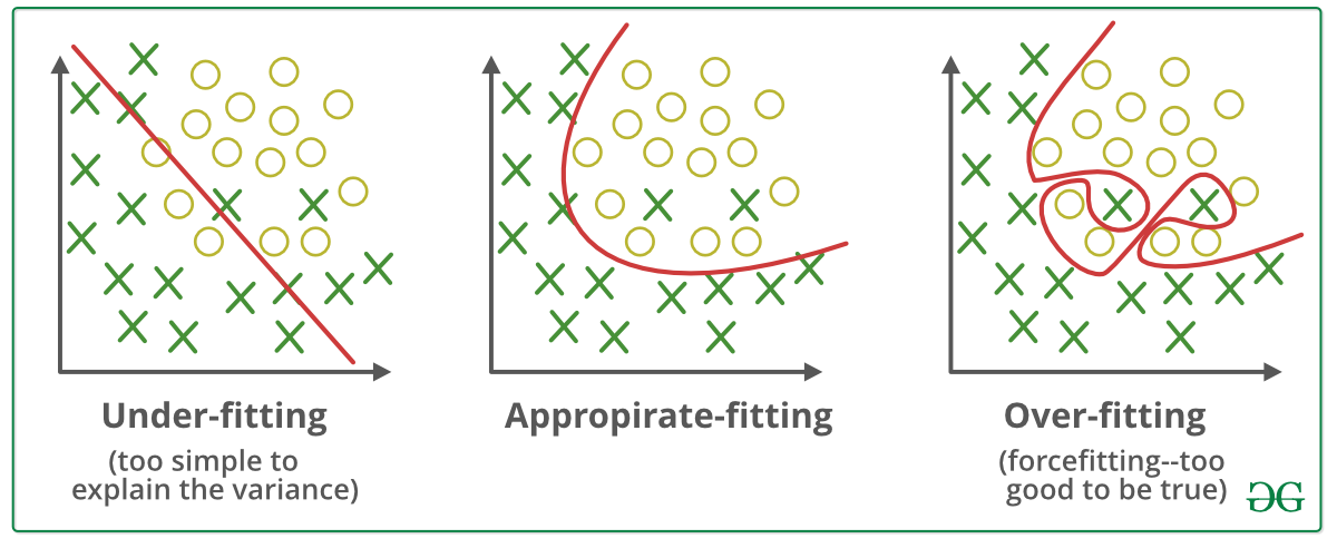
Bias (Underfitting): The error introduced by the model being too simple to capture the true patterns.
Variance (Overfitting): The error introduced by the model being too complex and capturing noise/outliers specific to the training data.
Underfitting (High Bias)#
Definition: The model is too simple and fails to learn the basic patterns.
Indicator: Low accuracy on both Training and Test data.
In KNN: Caused by a very large \(k\). The model is too constrained by averaging too many points.
Underfitting vs Overfitting#
Type |
Description |
Visual Intuition |
|---|---|---|
Underfitting |
Model too simple — fails to capture patterns |
High train & test error |
Overfitting |
Model too complex — memorizes training data |
Low train, high test error |
Overfitting (High Variance)#
Definition: The model learns the training data too well, memorizing noise instead of general rules.
Indicator: Very High Training Accuracy, but Significantly Lower Test Accuracy.
In KNN: Caused by a very small \(k\) (e.g., \(k=1\)). The boundary is too complex and sensitive to noise.
The key is to adjust the model’s complexity (like changing \(k\)) to maximize Generalization (Test Accuracy) without sacrificing too much Training Accuracy.

Back to KNN: Understanding the KNN Decision Boundary#
K-Nearest Neighbors (KNN) is an instance-based learning algorithm.
It doesn’t build an explicit mathematical model — instead, it classifies new points based on the majority vote of their k nearest neighbors.
Each point is classified by looking at its neighbors in the feature space.
Decision boundaries are formed where the majority class changes — often resulting in non-linear, curved boundaries.
As k increases, the boundary becomes smoother (less sensitive to noise).
Let’s visualize how KNN creates these boundaries using two features of the Iris dataset.
# --- Visualizing KNN Decision Boundaries ---

import numpy as np
import matplotlib.pyplot as plt
from sklearn.neighbors import KNeighborsClassifier
from sklearn.datasets import load_iris
from matplotlib.colors import ListedColormap

# Load data
iris = load_iris()
X = iris.data[:, :2]  # Use only first two features for easy visualization
y = iris.target

# Train KNN model
knn = KNeighborsClassifier(n_neighbors=5)
knn.fit(X, y)

# Create a mesh grid (like pixels for the background)
x_min, x_max = X[:, 0].min() - 1, X[:, 0].max() + 1
y_min, y_max = X[:, 1].min() - 1, X[:, 1].max() + 1
xx, yy = np.meshgrid(np.arange(x_min, x_max, 0.02),
                     np.arange(y_min, y_max, 0.02))

# Predict class for each point in mesh grid
Z = knn.predict(np.c_[xx.ravel(), yy.ravel()])
Z = Z.reshape(xx.shape)

# Define color maps
cmap_light = ListedColormap(['#FFAAAA', '#AAFFAA', '#AAAAFF'])
cmap_bold  = ListedColormap(['#FF0000', '#00FF00', '#0000FF'])

# Plot decision boundary
plt.figure(figsize=(8, 6))
plt.contourf(xx, yy, Z, cmap=cmap_light)

# Plot training points
plt.scatter(X[:, 0], X[:, 1], c=y, cmap=cmap_bold, edgecolor='k', s=50)
plt.title("🌸 KNN Decision Boundary (k = 5)")
plt.xlabel("Sepal length (cm)")
plt.ylabel("Sepal width (cm)")
plt.show()
/opt/hostedtoolcache/Python/3.11.14/x64/lib/python3.11/site-packages/IPython/core/pylabtools.py:170: UserWarning: Glyph 127800 (\N{CHERRY BLOSSOM}) missing from font(s) DejaVu Sans.
  fig.canvas.print_figure(bytes_io, **kw)
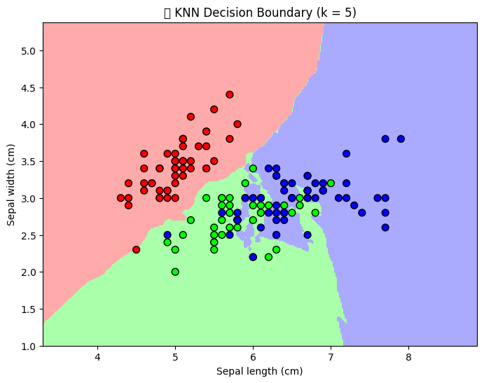
💬 Discussion:
Notice how the colored regions represent KNN’s decision boundaries — areas where the algorithm assigns new samples to a specific class.
The boundaries are flexible and follow the data — unlike linear models.
Use our Interative Visualization, try changing
n_neighbors(e.g., 1, 3, 10) to see how it affects the smoothness of boundaries.