Conditional Probability: Updating Beliefs With Context#
Now consider the weather again.
You hear there is a 30 percent chance of rain today. Later, you look outside and see dark clouds gathering.
Your belief changes.
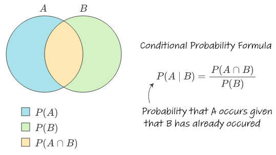
This adjustment is captured by conditional probability, which answers questions of the form:
What is the probability of an event, given that something else has already happened?
In data science, conditional probability appears constantly:
the probability of disease given a positive test
the probability a user clicks given that they saw an ad
the probability of fraud given unusual account activity
We rarely reason in isolation. We reason with context.
Mathematically: Conditional Probability
If \(P(B) > 0\), the conditional probability of \(A\) given \(B\) is
\(P(A \mid B) = \frac{P(A \cap B)}{P(B)}\)
This formula says:
among all outcomes where \(B\) happens, what fraction also satisfy \(A\)?
An event \(A\) and its complement \(A^c\) together cover the entire sample space \( \Omega \). Source: Stack Overflow
Small Python Simulation#
Example: rolling a die
\(A\): the roll is even
\(B\): the roll is greater than 3
import numpy as np

np.random.seed(0)

n = 100_000
rolls = np.random.randint(1, 7, size=n)

A = (rolls % 2 == 0)    # even
B = (rolls > 3)         # 4, 5, 6

p_B = B.mean()
p_A_and_B = (A & B).mean()
p_A_given_B = p_A_and_B / p_B

print("P(B) ≈", p_B)
print("P(A ∩ B) ≈", p_A_and_B)
print("P(A | B) ≈", p_A_given_B)
P(B) ≈ 0.50297
P(A ∩ B) ≈ 0.33429
P(A | B) ≈ 0.6646320854126487
In data science, we often observe evidence first and then ask what it tells us about an underlying cause.
Examples:
A medical test comes back positive — how likely is the disease?
An email looks suspicious — how likely is it spam?
A model flags an anomaly — how likely is it fraud?
Bayes’ theorem formalizes how beliefs should change when new evidence appears.
It tells us how to update our beliefs when new information arrives.
Bayes’ theorem connects four key ideas:
what we believed before seeing data
how likely the evidence is
how common the event is overall
what we should believe after seeing the evidence
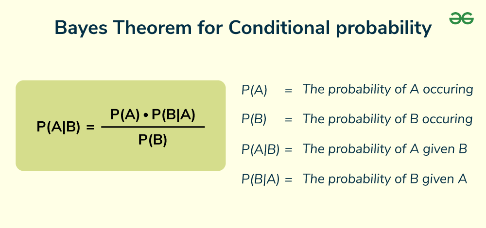
Mathematically: Bayes’ Theorem
If \(P(B) > 0\), then
\(P(A \mid B) = \dfrac{P(B \mid A)\,P(A)}{P(B)}\)
where:
\(P(A)\) is the prior (what we believed before seeing data)
\(P(B \mid A)\) is the likelihood
\(P(A \mid B)\) is the posterior (updated belief)
Bayes’ theorem reveals an important lesson. Evidence alone is not enough. A positive test result does not automatically mean something is likely. The background rate matters just as much as the test accuracy.
This is why Bayes’ theorem is both powerful and humbling. It forces us to confront our assumptions and reminds us that context shapes meaning.
Crucially, Bayes reminds us that evidence must be interpreted in context. A strong signal does not guarantee a likely cause if the cause itself is rare.
Data Science Connection: Bayes’ theorem underlies:
- Naive Bayes classifiers
- Probabilistic reasoning in ML
- Model calibration and uncertainty interpretation
Small Python Simulation#
Example: medical testing and base rates
1% of the population has a condition
The test detects it 95% of the time
The test gives false positives 5% of the time
# Example numbers for illustration (not medical advice)

p_disease = 0.01
p_positive_given_disease = 0.95
p_positive_given_no_disease = 0.05

p_no_disease = 1 - p_disease

# Total probability of testing positive
p_positive = (
    p_positive_given_disease * p_disease +
    p_positive_given_no_disease * p_no_disease
)

# Bayes' theorem
p_disease_given_positive = (
    p_positive_given_disease * p_disease
) / p_positive

print("P(Disease) =", p_disease)
print("P(Positive) =", p_positive)
print("P(Disease | Positive) =", p_disease_given_positive)
P(Disease) = 0.01
P(Positive) = 0.059000000000000004
P(Disease | Positive) = 0.16101694915254236