Introduction: What is Natural Language Processing?#
Natural Language Processing (NLP) is a subfield of Artificial Intelligence (AI) and Computational Linguistics focused on enabling machines to understand, interpret, and generate human language in a valuable way. As the primary mode of human communication, natural language is rich, nuanced, and often ambiguous. NLP bridges the gap between human language and machine-understandable formats, enabling a wide range of applications, from automated translation systems to intelligent chatbots and sentiment analysis engines.
In simple terms:
NLP teaches machines how to read, listen, understand, and talk like humans, or at least as close as we can get.
With the rapid growth of digital data—emails, social media posts, news articles, product reviews, and more—NLP has become a cornerstone technology in data-driven decision-making. NLP combines techniques from computer science, linguistics, and machine learning to process and analyze large amounts of natural language data. Advances in machine learning and deep learning have pushed NLP from rule-based systems to state-of-the-art models capable of reasoning with context, tone, and semantics. Applications of NLP include:
Machine Translation (e.g., Google Translate)
Sentiment Analysis (e.g., analyzing product reviews)
Chatbots & Virtual Assistants (e.g., Siri, Alexa)
Text Summarization (e.g., news article summarization)
Speech Recognition (e.g., voice-to-text transcription)
19.1 The Importance of NLP#
Language is the primary medium of human communication, making NLP essential for bridging the gap between humans and machines. Key reasons for its importance include:
Automation of Text Processing: Reduces manual effort in analyzing documents, emails, and reports.
Enhancing Human-Computer Interaction: Enables voice assistants and chatbots to respond naturally.
Business Intelligence: Helps companies analyze customer feedback, social media trends, and market sentiments.
Accessibility: Powers tools like speech-to-text for the hearing impaired and language translation for global communication.
19.2 Historical Evolution of NLP#
###19.2.1 Early Rule-Based Systems (1950s–1980s)
NLP began in the 1950s with a focus on symbolic approaches. Early researchers developed rule-based systems where grammar rules were manually coded. For example, machine translation systems like the Georgetown-IBM experiment (1954) translated a few Russian sentences into English using a small set of linguistic rules.
Challenges:
High maintenance effort
Poor adaptability to new domains
Limited understanding of context
19.2.2 Statistical NLP (1990s–2010s)#
With the availability of large datasets and increased computational power, NLP shifted toward statistical models. Probabilistic approaches, such as n-gram language models, Bayesian classifiers, and Hidden Markov Models (HMMs), became popular. These methods learned patterns from text data instead of relying solely on hand-written rules.
Key advantages:
Better scalability
Adaptation to multiple domains
Limitations remained in handling long-term dependencies and semantic understanding.
19.2.3 Neural NLP and Deep Learning Era (2013–Present)#
The advent of deep learning revolutionized NLP. Recurrent Neural Networks (RNNs) and Long Short-Term Memory (LSTM) networks improved the modeling of sequential data. Later, transformer architectures—introduced in “Attention Is All You Need” (2017)—enabled massive improvements in tasks like translation, summarization, and question answering. Pre-trained language models such as BERT, GPT, and T5 have since set new benchmarks across nearly all NLP tasks.
19.4 Fundamental NLP Tasks: Pipeline of NLP#
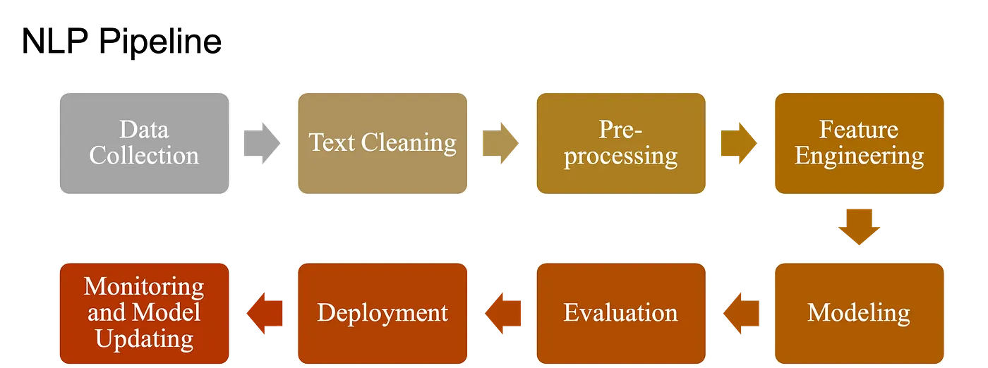
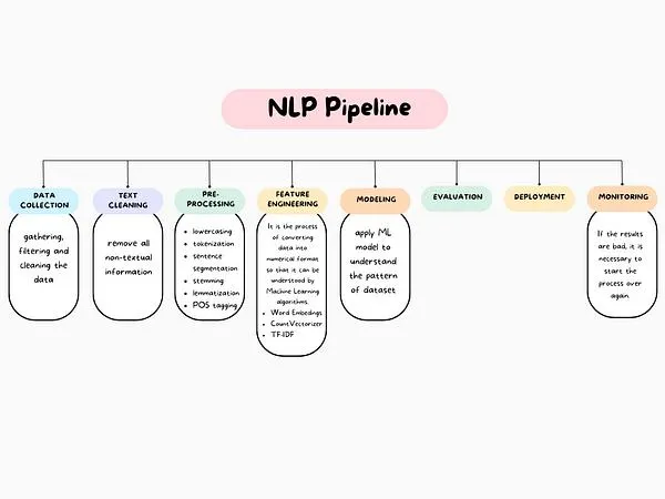
NLP covers a broad range of tasks. Some are foundational building blocks; others are application-focused. The Natural Language Processing (NLP) pipeline includes:
Raw Data (documents/text) Collection
Text Preprocessing
Basic Preprocessing: Text cleaning, Tokenizatuon, Stemming etc.
Advanced Preprocessing: POS tagging etc.
Feature Extraction/Engineering
ML Modeling
Evaluation, Deployment and Monitoring

19.4.0. Data Acquisition/ Raw Data Collection#
The first step in NLP is to obtain the raw text data in the form of documents, such as tweets, articles, reviews.
Basic Preprocessing:#
19.4.1. Text Preprocessing#
Before analysis, raw text must be cleaned and structured. That is why, in this step, the raw text is pre-processed by performing various operations such as tokenization, stop-word removal, stemming, and lemmatization, etc. This step is important as it helps to clean and normalize the data, making it easier to work.
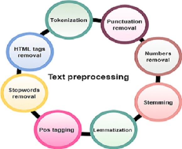

Text Cleaning: Removing noise, unwanted symbols, and irrelevant data.
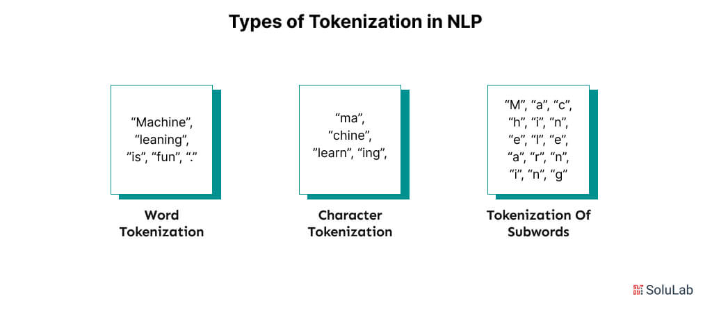
Tokenization: Splitting text into words or subwords (making it easier for machines to process). Example: “I love NLP!” → [“I”, “love”, “NLP”, “!”]

There can be different type of tokenizations:
Stopword Removal: (Filtering out common words (e.g., “the,” “is”)) It involves identifying and removing common words such as “the”, “a”, “an”, “and”, “of”, that are unlikely to carry significant meaning in the text. These words are commonly referred to as “stop words” because they can be “stopped” or removed without affecting the overall meaning of the text.

Stemming & Lemmatization: Reducing words to their base forms (e.g., “running” → “run”).
Stemming: Remove affixes from a word to get base form (stem) of a word (stem might not be a lexicographically correct word). Example: “running” → “run” (rough cut). Good for search engines and simple tasks.
Lemmatization: Find lemma (dictionary form) of a inflected word (a lemma is always a lexicographically correct word). Example: “running” → “run” (dictionary-based, more precise). Best for tasks where meaning and context are important, like text classification and sentiment analysis.
Lowercasing and Normalization: Ensuring consistent text representation.
Handling Punctuation & Numbers:: Remove or normalize.
Spell Correction: Fix typos (“NLP is awsome” → “awesome”).
Special Character Removal: Remove punctuation (e.g., “Hello!” → “Hello”), numbers, emojis (or converting emojis into textual descriptions), HTML tags (e.g., “good” → “good”), and other non-alphabetic symbols. Extra spaces, tabs, and formatting characters are also cleaned to ensure uniform text.
Advanced Preprocessing:#
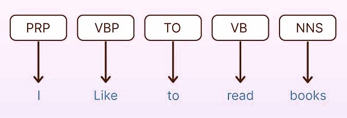
Part-of-Speech (POS) Tagging: is the process of assigning grammatical labels (lexical category) to each word in a sentence, such as noun, verb, adjective, or preposition. For example, in the sentence “The quick brown fox jumps over the lazy dog,” the words would be tagged as follows: “The” as a determiner, “quick” and “brown” as adjectives, “fox” and “dog” as nouns, “jumps” as a verb, and “over” as a preposition.
Some Common POS Tags: NN (Noun), VB (Verb), JJ (Adjective), RB (Adverb), PRP (Pronoun), IN (Preposition) and DT (Determiner).
Why It Matters:
Helps machines understand sentence structure (grammar).
Essential for lemmatization (reducing words to their base forms).
Improves text analysis in tasks like parsing, translation, and sentiment analysis.
Named Entity Recognition (NER): Finding names of people, organizations, locations, etc.
Dependency Parsing: Understanding grammatical relationships between words.
19.4 Text Representation and Feature Extraction/Representation (Turning texts into vectors)#
Machines cannot directly understand raw text; it must first be transformed into a numerical format. Feature extraction is the process of converting text into numerical representations—such as vectors capturing word frequencies or semantic meanings—so that machine learning models can interpret and use them for tasks such as sentiment analysis, classification, or translation.
There are several common approaches to representing text numerically:
19.4.1 Bag-of-Words (BoW)#
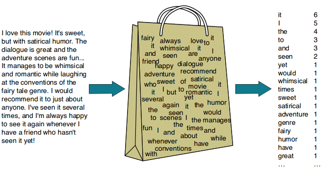
The Bag-of-Words (BoW) model is one of the simplest and most widely used text representation techniques. It represents text by counting the occurrences of each word in the document, completely ignoring grammar, word order, and context.
Concept: Treats each document as a “bag” of words—only the words themselves and their counts matter, not the order in which they appear.
Steps to follow:
Tokenize the text (split into words).
Build a vocabulary of all unique words across the corpus.
Count the frequency of each word in each document.
Why? Each document is transformed into a vector where each position corresponds to a word in the vocabulary and the value is the frequency (count) of that word in the document.
Example:
Document: “Hi. This is an example sentence in an Example Document.”
Tokenization (lowercased, punctuation removed):
[hi, this, is, an, example, sentence, in, an, example, document]
Vocabulary: [hi, this, is, an, example, sentence, in, document]
Word Frequencies in the document: [1, 1, 1, 2, 2, 1, 1, 1]
Word Frequencies in the document: [1, 1, 1, 2, 2, 1, 1, 1]→ corresponds to the order of the vocabulary.
So the BoW vector for this document is: [1, 1, 1, 2, 2, 1, 1, 1]
More Example(s):

Advantages: Simple and fast, works well for basic text classification.
Limitations: Ignores meaning and word order, produces sparse vectors with many zeros for large vocabularies. As vocabulary size can grow rapidly, increasing memory usage.
19.4.2 N-grams#
BoW consider individual words (unigrams), but language meaning often depends on word combinations. N-grams are a variation of Bag of Words that captures sequences of N adjacent words.
Types:
Unigram: single words (“machine”, “learning”)
Bigram: pairs of words (“machine learning”)
Trigram: triples (“natural language processing”)
Example:

N-grams help models understand phrases and partial word order, improving performance in many tasks. Still it has some limitation such as larger n can create exponentially larger vocabulary, rare phrases may not generalize well,etc.
19.4.3 TF-IDF (Term Frequency-Inverse Document Frequency)#
While BoW treats all words equally, TF-IDF weighs words based on how important they are to a document relative to a collection (corpus) of documents.
TF-IDF assigns more weight to informative words that are frequent in a specific document but rare across the corpus. This helps downweight common words like “the” or “is.”
####Formula(s):
Term Frequency (TF): How often a word appears in a document.
Document Frequency (DF): Number of documents that contain the term.
where (n_t) is the number of documents containing term (t).
Inverse Document Frequency (IDF): How rare a word is across all documents.
where (N) is the total number of documents.
TF–IDF:
Words that appear frequently in one document but rarely in others get higher weights, highlighting their importance. This helps reduce the impact of common words like “the” or “is” that appear everywhere.
Example: Calculating DF, IDF (base-10), TF, and TF–IDF
We have 3 documents:
machine learning is funmachine learning is powerfuldeep learning powers AI
Vocabulary:
$\(
[\text{machine}, \text{learning}, \text{is}, \text{fun}, \text{powerful}, \text{deep}, \text{powers}, \text{ai}]
\)$
Step 1 — Document Frequency (DF)#
DF counts how many documents contain the term:
Step 2 — Inverse Document Frequency (IDF)#
Using log base 10 (to match the numeric examples):
So:
(Interpretation: rarer terms → larger IDF.)
Step 3 — Term Frequency (TF)#
For a term (t) in document (d):
Example for Doc 1 (“machine learning is fun”):
Total terms in Doc1 = 4.
Step 4 — TF–IDF#
For Doc 1:
(Despite equal TF in Doc1, “fun” scores higher because it is rarer across the corpus.)
Observation:
Even though “machine” and “fun” occur the same number of times in Doc 1, “fun” has a higher TF–IDF score because it is rarer in the overall corpus.
More Example(s):

19.4.4 Word Embeddings#
Traditional frequency-based methods treat each word as independent, but words have semantic relationships. Word embeddings map words into dense vectors in a continuous space, where similar words lie close together.
Popular algorithms include: Word2Vec, GloVe
These embeddings capture relationships like: vector(“king”) – vector(“man”) + vector(“woman”) ≈ vector(“queen”)
19.4.5 Contextual Embeddings#
Unlike static embeddings (Word2Vec, GloVe), contextual embeddings generate word representations based on surrounding words, capturing meaning that depends on context. For example, the word “bank” in “river bank” vs. “bank account” will have different embeddings.
Modern NLP models such as BERT and GPT produce contextual embeddings, enabling them to understand nuances and disambiguate meanings dynamically.
19.3 The Challenge of Human Language#
Despite advancements, NLP faces several challenges due to the complexity of human language. Understanding human language is much harder than processing numbers or images. Why? Because language is messy.
Key Challenges in NLP#
Despite advancements, NLP faces several challenges due to the complexity of human language:
1. Ambiguity#
Type |
Description |
Example |
|---|---|---|
Lexical Ambiguity |
Words with multiple meanings. |
“Bank” (financial institution vs. river edge) |
Syntactic Ambiguity |
Sentence structures with multiple interpretations. |
“I saw the man with the telescope” (who had the telescope?) |
Semantic Ambiguity |
Phrases requiring context for disambiguation. |
“Time flies like an arrow” (time moves quickly vs. insects resembling arrows?) |
2. Context Understanding:#
Sentences change meaning based on situation. E.g., cold ice cream vs. cold soup.
Human language depends on tone, sarcasm, and cultural references, which are hard for machines to interpret.
Example:
Sincere: “That was a great movie!” (positive)
Sarcastic: “That was a great movie…” (negative, with ironic tone)
3. Slang & Informal Text#
Handling emojis, abbreviations (e.g., “BRB,” “LOL”).
4. Data Sparsity & Rare Words#
Problem: Many words appear infrequently in training data, making it hard for models to learn their meanings.
Solutions:
Subword Tokenization: Break words into smaller units (e.g., Byte Pair Encoding)Pre-trained Embeddings: Use models like Word2Vec or GloVe
5. Multilingual & Low-Resource Languages#
Problem: Bias toward high-resource languages (English, Chinese)as most NLP models are trained on these high-resource languages, leaving many languages underrepresented.
Solutions:
Multilingual Models: mBERT, XLM-RTransfer Learning: Adapt pre-trained models
6. Morphological Complexity#
Different languages have different grammar rules.
Language |
Challenge |
Example (Analysis) |
|---|---|---|
Finnish |
Agglutinative morphology |
“Talossanikin” = “talo-ssa-ni-kin” (house-in-my-too) |
Arabic |
Root-and-pattern system |
“كتب” (k-t-b) → “kataba” (wrote), “kitāb” (book) |
Turkish |
Vowel harmony |
“evlerimizde” (in our houses) → 4 suffixes |