Sample Space and Events: Defining the World#
Every probability problem starts by defining what could happen.
If you flip a coin once, there are only two possible outcomes: heads or tails. This complete set of possible outcomes is called the sample space.
If you flip a coin once, the possible outcomes are
{H, T}.
That complete list of outcomes is the sample space.
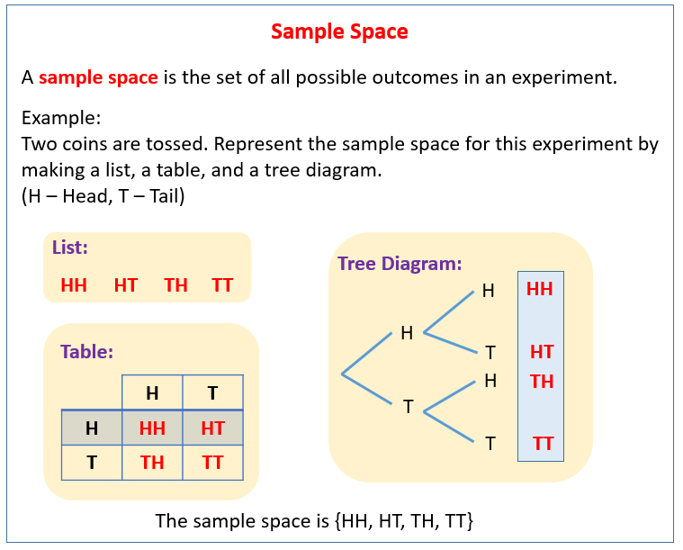
Sample Space illustration. Source: Online Math Learning.
An event is any subset of the sample space, something we care about.
For example:
the coin lands on heads
it rains tomorrow
a customer makes a purchase
Events can be simple or complex, but they always live inside the sample space. Probability asks a single guiding question:
How likely is this event to occur if the situation were repeated many times?
Mathematically
Let \(Ω\) be the sample space, the set of all possible outcomes.
An event \(A\) is a set such that \(A ⊆ Ω\).
Probability is a function \(P(·)\) that assigns a number to events.

The relationship between a sample space, events, and probabilities is often visualized using simple diagrams.
Assigning Probabilities to Events#
Once an event is defined, we assign it a number between 0 and 1.
\(P(A)\) represents the probability that event \(A\) occurs.
\(1 - P(A)\) represents the probability that event \(A\) does not occur (the complement of \(A\)).
For example, if \(A\) is the event “the coin lands on heads”:
\(P(A) = 0.5\)
\(1 - P(A) = 0.5\)
Together, an event and its complement account for all possible outcomes.
Before we start computing probabilities, we need a few basic rules that probabilities must obey.
The Rules of the Game: Probability Axioms#
Probability is not guesswork; it follows strict rules.
Probabilities are never negative
You cannot have a “−20% chance” of rain.Something must happen
The probabilities of all possible outcomes add up to 1.Mutually exclusive events add cleanly
If two events cannot happen at the same time, the probability of either happening is the sum of their probabilities.
These ideas are often called the axioms of probability.
They are assumed by all statistical and machine learning methods.
These rules ensure that probability behaves consistently and logically. Every model you build and every experiment you analyze rests on these foundations, even when the formulas are hidden.
Probability does not eliminate uncertainty; it helps us reason clearly in its presence.