18.2 Optimizers#
Optimizers are algorithms that adjust the weights of a neural network to minimize the loss function during training. Two most basic optimizers are
SGD (Stochastic Gradient Descent): Basic optimization
Adam: Adaptive learning rates (most popular)
Stochastic Gradient Descent (SGD) updates the model’s parameters by computing the gradient of the loss on a small batch of data and moving in the direction that reduces the loss. While simple and effective, SGD uses a fixed learning rate and can be slow to converge, especially for complex models.
To address these limitations, Adam (Adaptive Moment Estimation) is widely used due to its ability to adapt the learning rate for each parameter individually by combining the benefits of momentum and RMSProp optimizers. Adam often results in faster convergence and better performance without much tuning, making it the most popular choice for training deep neural networks.
Note: Momentum helps speed up learning by smoothing updates using past gradients, while RMSProp adapts learning rates based on recent gradient magnitudes. Adam combines both techniques for efficient and stable training.
Training Techniques & Regularization#
Training a neural network consists of two main steps performed repeatedly over many iterations: the forward pass and the backward pass.
Forward Pass#
During the forward pass, input data flows through the network, and the final output layer generates predictions \((\hat{y}^{(i)})\) for each input example (i). The network then computes the loss function (L), which quantifies the difference between predicted outputs and true targets \((y^{(i)}\)\). For a batch of (m) samples, the average loss is:
This loss guides how well the model is performing.
Here are the details of step by step:
Forward Pass: Step-by-Step#
The forward pass is the phase in which input data flows through the neural network to produce predictions.

Figure: Forward Pass in Neural Networks
Here’s how it works:
Input Layer
Each input example is denoted as \(x_i^{(0)}\) which is fed into the network.
Hidden Layers
For each hidden layer ( l = 1, 2, \ldots, L ), the network performs the following steps:
Linear transformation:
$\(
z_i^{[l]} = W^{[l]} x_i^{(l-1)} + b^{[l]}
\)$
Non-linear activation:
$\(
x_i^{(l)} = \sigma\left(z_i^{[l]}\right)
\)$
Here, ( x_i^{(l)} ) is the activated output of layer ( l ), used as input for the next layer.
Output Layer
After the last hidden layer ( L ), the output layer produces the final prediction:
$\(
\hat{y}_i = f\left(x_i^{(L)}\right)
\)$
where ( f ) is an appropriate output function (e.g., identity for regression, sigmoid for binary classification, softmax for multi-class classification).
Loss Computation
The predicted output \(\hat{y}_i\) is compared to the true label \(y_i\) using a loss function \(L(\hat{y}_i, y_i)\).
Example (Mean Squared Error):
$\(
L(\hat{y}_i, y_i) = (\hat{y}_i - y_i)^2
\)$
Average Loss Over the Batch
For a batch of ( m ) samples, the average loss is:
$\(
L = \frac{1}{m} \sum_{i=1}^m L(\hat{y}_i, y_i)
\)$
This average loss quantifies how well the model is performing and is used in the backward pass to update model parameters.
Click Here for Interactive Forward Propagation Visualization
Backward Pass (Backpropagation)#
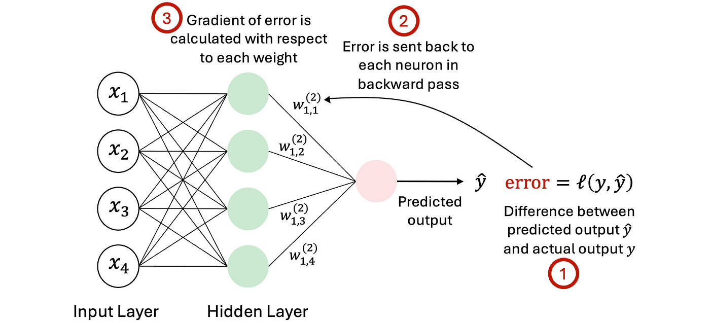
In the backward pass, gradients of the loss with respect to each parameter (weights \(W^{[l]}\) at layer \(l\)) are computed using the chain rule.
The chain rule lets us break down the gradient of the loss into simpler parts by following the flow of computations backward through the network. It helps calculate how changes in weights affect the final loss by multiplying the derivatives of each intermediate step.
Mathematically:
where:
\(a^{[l]}\) is the activation output of layer \(l\),
\(z^{[l]} = W^{[l]} a^{[l-1]} + b^{[l]}\) is the input to the activation function.
Weight Update
The weights are then updated using gradient descent:
where:
\(W^{[l]}\) = current weights at layer \(l\),
\(\alpha\) = learning rate (controls the step size),
\(\frac{\partial L}{\partial W^{[l]}}\) = gradient of the loss with respect to the weights.
Repeat
This process of forward pass, backward pass, and weight update is repeated over many epochs (full passes over the training data) until the error is minimized.

Figure: Backpropagation in Neural Networks
Click Here for Interactive Backpropagation Visualization
Regularization Techniques#
Regularization adds penalty terms to the loss function to prevent overfitting, which happens when the model learns the training data too well including noise, resulting in poor performance on new, unseen data. By constraining model complexity, regularization encourages the model to generalize better.
L2 Regularization (Weight Decay):#
L2 regularization adds the sum of the squared weights to the loss function. The hyperparameter \(\lambda\) controls the strength of this penalty. This encourages the model to keep weights small but not necessarily zero, which tends to distribute the “importance” across many features and reduces overfitting.
L1 Regularization:#
L1 regularization adds the sum of the absolute values of the weights to the loss. This tends to push some weights exactly to zero, effectively performing feature selection by encouraging sparsity in the model. This can be useful when you want a simpler model with fewer active features.
Why Use Regularization?#
Improves Generalization: By limiting the size or number of weights, the model avoids fitting noise and irrelevant patterns in the training data.
Controls Model Complexity: Prevents weights from growing too large, which can cause unstable predictions.
Feature Selection (L1): Helps identify and ignore irrelevant features by forcing their weights to zero.
Choosing \(\lambda\)#
The regularization strength \(\lambda\) is a hyperparameter that must be tuned carefully:
Too small: little effect on overfitting
Too large: model may underfit by being too constrained
Example: When to Use L1 vs. L2 Regularization#
L2 Regularization (Ridge):
Use when most features are relevant and you want to keep them all but reduce overfitting by shrinking weights smoothly.
Example: Predicting house prices using many meaningful features.L1 Regularization (Lasso):
Use when you expect only a few important features and want the model to ignore irrelevant ones by setting some weights exactly to zero.
Example: Selecting important genes from thousands of candidates in a biological study.
Other Common Regularization Methods (Brief)#
Dropout: Randomly sets some activations to zero during training to prevent co-adaptation of neurons, helping the model generalize better.
Early Stopping: Stops training when performance on a validation set stops improving, preventing overfitting.
Putting It All Together: How Neural Network Training Happens#
After understanding how regularization helps prevent overfitting and improve generalization, it’s important to see how the entire training process operates in practice. Training a neural network involves repeatedly feeding data through the model in manageable portions, updating parameters, and gradually improving performance.
The next section explains the key concepts of batch size, iteration, and epoch, which organize how training data is processed and how the model learns over time.
Neural Network Training: Batch Size, Iteration, and Epoch#
When training a neural network, the dataset is usually too large to process all at once, so it is split into smaller parts called batches.
Batch Size#
The number of training examples used in one forward and backward pass.
For example, a batch size of 32 means the model processes 32 samples before updating weights.
Iteration#
One update of the model’s parameters (weights and biases).
Each iteration uses one batch of data.
Epoch#
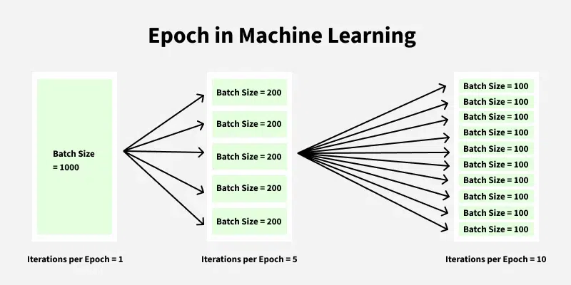
One full pass over the entire training dataset.
If the dataset has 1000 samples and batch size is 100, then:
$\(
1 \text{ epoch} = \frac{1000}{100} = 10 \text{ iterations}
\)$

Figure: Epoch in Machine Learning
Training Process Overview#
Start Training: Initialize model parameters.
For each epoch (repeat multiple times):
Divide data into batches according to batch size.
For each batch:
Perform forward pass to calculate predictions.
Calculate loss based on predictions and true labels.
Perform backward pass (backpropagation) to compute gradients.
Update weights using gradients (e.g., gradient descent).
Repeat until model performance stabilizes or desired accuracy is reached.

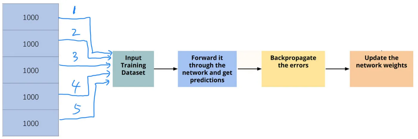
Figure: In the Input Training Dataset step, as different kinds of strategies, we can assign a Batch Size to determine how many training datasets are going to be used for one weights updating process. For example, there are 5000 images in total as the training datasets. If we set the Batch Size = 1000, we get 5 batches of training datasets. As a result, the weights updating process will be executed 5 times (Iterations).