Distance Metrics and Variants in KNN

Distance Metrics and Variants in KNN#

The choice of distance metric greatly influences how KNN defines “neighborhoods” and classifies points.
It depends on the nature of the data and the problem context.

Common Distance Metrics#

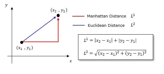
1. Euclidean Distance (L2 Norm)#

Detail	Description
Description	Measures the straight-line distance between two points in space.
Use When	Features are continuous and measured on the same scale. Differences in magnitude are meaningful (e.g., height, weight).
Caution	Highly sensitive to outliers and varying feature scales — always normalize or standardize data before use.
Formula	$$d(\mathbf{x}, \mathbf{y}) = \sqrt{\sum_{i=1}^{n} (x_i - y_i)^2}$$

2. Manhattan (City Block) Distance (L1 Norm)#

Detail	Description
Description	Measures the distance by summing absolute differences along each dimension (like moving along a grid).
Use When	Movement is restricted to orthogonal directions (e.g., city blocks). Features contribute independently to distance. Works better than Euclidean for high-dimensional data as it reduces the impact of large single-feature deviations.
Caution	Less sensitive to outliers than Euclidean, but still requires feature scaling for optimal performance.
Formula	$$d(\mathbf{x}, \mathbf{y}) = \sum_{i=1}^{n}

3. Hamming Distance#

Detail	Description
Description	Counts the number of features where two samples differ (mismatches between attribute values).
Use When	Data is categorical or binary (e.g., yes/no, text encodings, DNA sequences).
Caution	Only works for discrete or categorical features. It gives a binary measure (different or not different) for each feature.
Formula	$$d(\mathbf{x}, \mathbf{y}) = \sum_{i=1}^{n} \mathbb{I}(x_i \neq y_i)$$ (Where $\mathbb{I}(\cdot)$ is the indicator function.)

4. Cosine Similarity#

Detail	Description
Description	Measures the cosine of the angle between two vectors — focuses purely on orientation, not magnitude or size.
Use When	Direction matters more than size (e.g., text analysis, where document length shouldn’t bias similarity). Common in recommender systems.
Caution	Returns similarity (1 is close, 0 is far) rather than distance. It is often converted to a distance metric as: $d = 1 - \text{similarity}$.
Formula	$$\text{Similarity}(\mathbf{x}, \mathbf{y}) = \frac{\mathbf{x} \cdot \mathbf{y}}{\|\mathbf{x}\| \|\mathbf{y}\|}$$

Weighted KNN#

So far, we have talked about standard KNN, where every one of the k neighbors has an equal vote. Now, we will introduce Weighted K-Nearest Neighbors changes this by giving more weight to the neighbors that are closer to the new data point.

Why? According to Weighted KNN, closer neighbors have a stronger influence on the prediction.

Mathematically, each neighbor is weighted by:

\[ w_i = \frac{1}{d_i + \varepsilon} \]

Where:

\[ d_i \text{ = distance between the query point and the } i^{\text{th}} \text{ neighbor} \]

\[ \varepsilon \text{ = a small constant to prevent division by zero} \]

This means points closer to the query point contribute more to the prediction than distant ones.

In scikit-learn, you can enable this using:

KNeighborsClassifier(n_neighbors=5, weights='distance')

Key Points to remember:

Standard KNN treats all neighbors equally (weights=’uniform’).
Weighted KNN emphasizes closer neighbors, making the classifier more robust to noise.
Works best when your features are continuous numeric values (like Iris measurements).-

Section 6: Ethics and Responsible ML#

Why Ethics Matter#

Machine Learning models can impact real people — from job applications to healthcare decisions. Therefore, fairness and transparency are essential.

Bias: When data reflects historical prejudice.
Fairness: Ensure models treat groups equally.
Transparency: Explain how the model makes decisions.
Privacy: Respect individuals’ personal data.

Example: A hiring model should not unfairly prefer one gender or race.

Section 7: Hands-on Practice#

Task: Identify the ML Type#

Predicting house prices → ?
Grouping customers → ?
Teaching a robot to play chess → ?

Section 8: Reflection Questions#

What distinguishes Machine Learning from traditional programming?
Why is testing important after training a model?
How can bias in ML models be reduced?

Summary: What We Learned#

In this chapter, we walked through the complete Machine Learning workflow — from data to deployment-ready model (conceptually).

We covered:

Understanding the dataset – explored real data (Iris flower dataset).
Defining features and labels – identified what to predict and what to use for prediction.
Training a model – taught a KNN to learn from data.
Evaluating performance – measured accuracy on unseen test data.
Visualizing data – saw how features relate and form clusters.

Key takeaway:
Machine Learning is about teaching computers to learn from data and improve over time — not just follow fixed rules.

ML enables systems to learn from data automatically.
Three main types: Supervised, Unsupervised, and Reinforcement.
Workflow: Data → Model → Evaluation → Deployment.
Ethical ML ensures fairness, transparency, and accountability.