Information Gain (IG)#
Once we know how to calculate Entropy, we can measure how much uncertainty (or impurity) is reduced when we split a dataset using a feature. This reduction is called Information Gain.
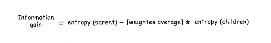
Information Gain measures the reduction in entropy achieved by a split. It tells us how much uncertainty (impurity) is removed by a particular split.
Definition#
Formally, suppose a split divides the parent node \(S\) into \(V\) subsets:
$\(
S_1, S_2, ..., S_V
\)$
Let:
\(|S|\) = total number of samples in the parent node
\(|S_v|\) = number of samples in child node \(S_v\)
Information Gain for a feature A is defined as:
where:
\(S\) = parent node (original dataset)
\(A\) = feature used for splitting
\(S_v\) = subset of \(S\) corresponding to value \(v\) of feature \(A\)
\(|S|\), \(|S_v|\) = number of samples in \(S\) and \(S_v\), respectively
The algorithm selects the feature with the highest Information Gain for splitting.
Intuition#
Information Gain measures how much a split reduces impurity:
A high IG means the feature created purer subsets (good split).
A low IG means the feature did not reduce impurity much (poor split).
Decision Trees choose the feature with the highest Information Gain at each step.
Example#
Suppose a dataset has 10 samples:
6 Pass, 4 Fail
Then the initial (parent) entropy is:
Now we split based on Feature A (e.g., “Study Hours”) which has two possible values:
A = High: 5 samples → 4 Pass, 1 Fail
A = Low: 5 samples → 2 Pass, 3 Fail
Compute entropy for each group:
Then the weighted average entropy after splitting is:
Finally, the Information Gain is:
So, splitting on Feature A reduces uncertainty by 0.124 bits.
Additional Example:#
Example illustrating the calculation of information gain. Source: Hendler 2018, slide 46.

Try it Yourself#
If you have another feature B that splits the same data into:
B = Yes: 6 samples (5 Pass, 1 Fail)
B = No: 4 samples (1 Pass, 3 Fail)
Try calculating:
Which feature gives a higher Information Gain — A or B?
import math

def entropy(class_counts):
    """
    Compute entropy for a list of class counts.
    class_counts: list of counts for each class
    """
    total = sum(class_counts)
    entropy_value = 0
    for count in class_counts:
        if count == 0:  # avoid log(0)
            continue
        p = count / total
        entropy_value -= p * math.log2(p)
    return entropy_value

def information_gain(parent_counts, split_counts_list):
    """
    Compute Information Gain.
    parent_counts: list of counts in the parent node
    split_counts_list: list of lists, each sublist contains counts in a child node
    """
    total_parent = sum(parent_counts)
    parent_entropy = entropy(parent_counts)

    weighted_entropy = 0
    for counts in split_counts_list:
        weight = sum(counts) / total_parent
        weighted_entropy += weight * entropy(counts)

    ig = parent_entropy - weighted_entropy
    return ig

# Example: Feature A split
# Parent node: 6 Pass, 4 Fail
parent = [6, 4]

# Feature A splits:
# High: 4 Pass, 1 Fail
# Low: 2 Pass, 3 Fail
split_A = [[4, 1], [2, 3]]

print("Information Gain for Feature A:", round(information_gain(parent, split_A), 3))

# Feature B splits:
# Yes: 5 Pass, 1 Fail
# No: 1 Pass, 3 Fail
split_B = [[5, 1], [1, 3]]

print("Information Gain for Feature B:", round(information_gain(parent, split_B), 3))
Information Gain for Feature A: 0.125
Information Gain for Feature B: 0.256