Introduction#
In the previous chapter, we explored the foundational concepts behind neural networks and saw how they can approximate functions using layers of interconnected neurons. However, standard feedforward networks struggle with high-dimensional data like images, where preserving spatial relationships is essential. We now shift our focus to Convolutional Neural Networks (CNNs), a specialized type of neural network designed to process and interpret image data effectively.
CNNs revolutionized the field of computer vision and are now the backbone of many modern applications, including facial recognition, medical image analysis, and autonomous driving.
Unlike fully connected neural networks, CNNs leverage three key ideas:
Local Receptive Fields (Convolution operations)
Parameter Sharing (Reduces the number of trainable weights)
Spatial Hierarchies (Pooling layers for downsampling)
These properties make CNNs translation-invariant and computationally efficient compared to dense neural networks when dealing with high-dimensional data like images.
19.1 Why Not Use Fully Connected Networks for Images?#
Consider a grayscale image of size 28×28 pixels. If we treat this as a flat input vector to a dense network, it results in 784 input nodes. For a 100x100 image, the number of inputs jumps to 10,000! Fully connected networks don’t scale well and tend to ignore spatial hierarchies like “edges” or “patterns.”
CNNs solve this by leveraging local connectivity, weight sharing, and spatial hierarchies to detect meaningful patterns in images.
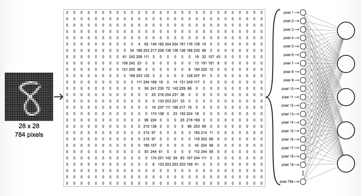
Figure: Fully connected networks flatten images into vectors, losing important spatial relationships like shape, texture, and position. This may work for simple images but fails on complex ones with pixel dependencies. CNNs preserve spatial information by using filters, making them more effective for image tasks like recognition and detection.
19.2 CNN Architecture Overview#
A typical CNN consists of the following layers:
Convolutional layer(s): Extracts features from the input dataset using learnable filters known as kernels applied to input images.
Pooling layer(s): Reduces the spatial dimensions of the input volume, speeding up computation, reducing memory usage, and helping prevent overfitting.
Fully connected layer(s): Used for the final classification or regression task.
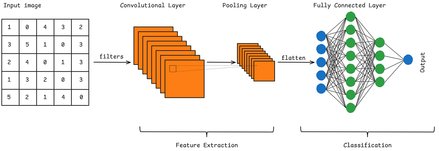
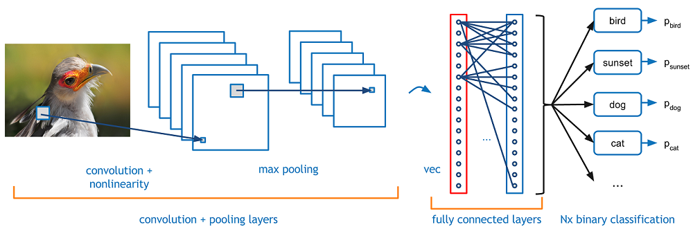
Figure: A simplified scheme of a simple CNN (with an example).
These layers are often supplemented with dropout and batch normalization for improved training stability.
19.2.1 Convolution Layer#
The convolutional layer is the core building block of a CNN. It applies a set of learnable filters (kernels) to the input, each detecting different features such as edges, textures, or patterns. A convolution operation refers to sliding a filter across the input image and computing the dot product between the filter weights and the corresponding input region. This operation produces a feature map (also known as activation map) that highlights where the detected feature appears in the input.
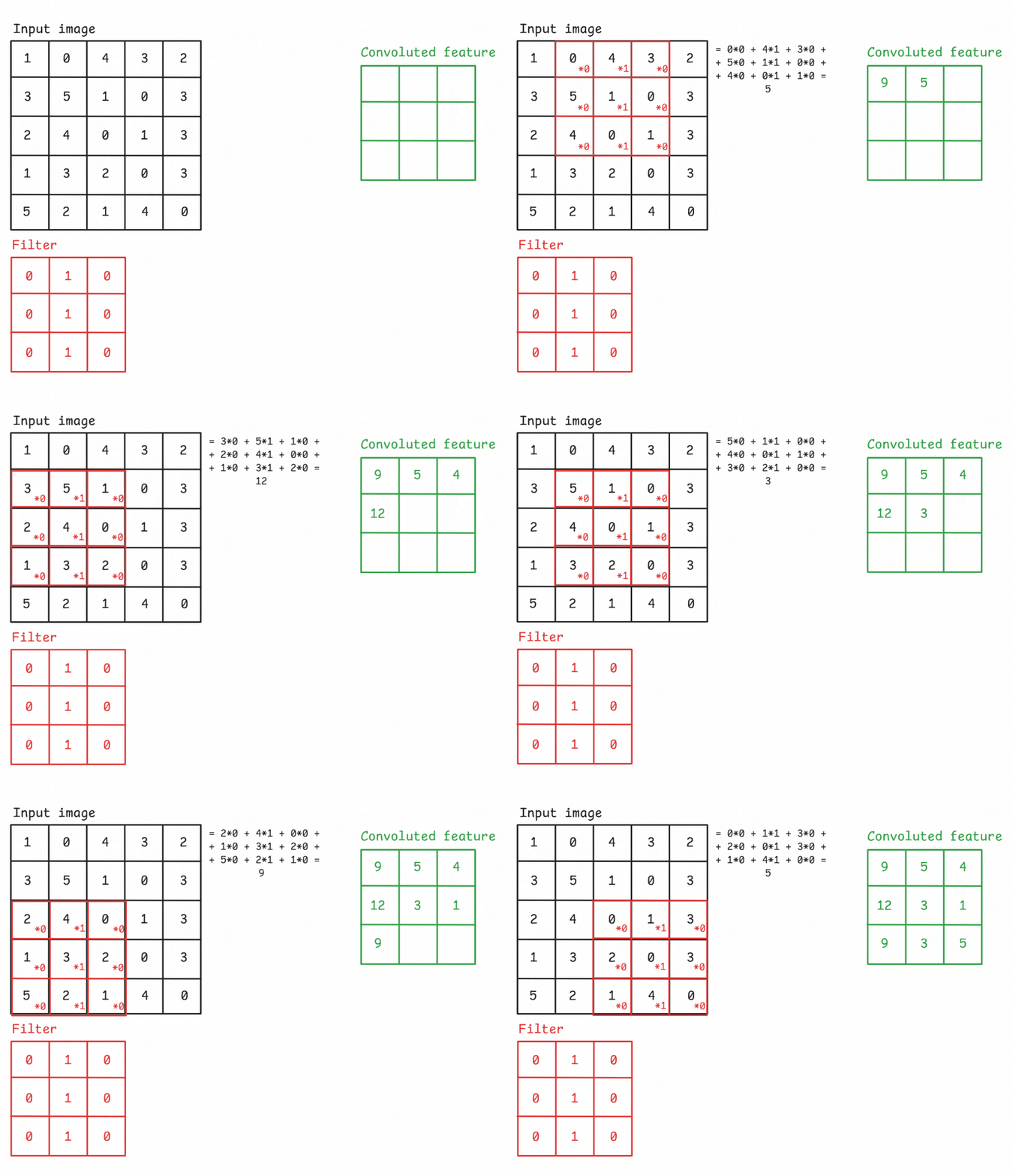
Figure: An example of a convolution operation applied to a 5×5 pixel, single-channel image using a 3×3 filter.
A Filter, or Kernel: in a CNN, is a small matrix used in the convolution operation. It’s a set of learnable weights that are applied to the input data to produce the output feature map. These small matrix of weights slides over the input data (such as an image), performs element-wise multiplication with the part of the input it is currently on, and then sums up all the results into a single output pixel. This process is known as convolution. Kernels are the key elements that allow CNNs to automatically learn spatial hierarchies of features within the input data. In image processing, a kernel might be a small matrix like 3x3 or 5x5.
Remember that, the filter values are trainable parameters, much like weights in a standard neural network. These values of the filters are learned during training through backpropagation, similar to weights in a traditional neural network. By sharing weights across the entire image, CNNs drastically reduce the number of parameters while retaining spatial information. The network learns multiple filters at each layer, each specialized to detect different features in the image, such as vertical edges, corners, or more complex textures.
There are some key parameters in a convolutional layer that include:
Kernel size (e.g., 3×3 or 5×5), which determines the receptive field.
Stride, the step size with which the filter moves across the image. A stride of 1 moves pixel-by-pixel, while a larger stride reduces spatial dimensions.
Padding, Controls whether we allow the output size to shrink or keep it the same as the input. It allows to adds extra pixels (usually zeros) around an image before convolution. It helps control the output size and preserves edge information.
Paddings are two types:
Same padding: Adds zeros so that the output has the same spatial dimensions (height and width) as the input. This helps preserve the size of the image throughout convolutional layers (same padding keeps the output the same size as the input, making it easier to stack many layers without losing resolution or cutting off edge information). Example: 5×5 input → 5×5 output (3×3 kernel, stride=1).
Valid padding: Adds no padding, so the convolution is only applied where the filter fully overlaps the input. This causes the output to shrink in size compared to the input. Example stride=1: 5×5 input → 3×3 output (3×3 kernel).
Remember: Higher strides = faster dimension reduction = less computation but potentially losing information.
Feature Map Size Calculation:#
The output spatial size (height or width) of a feature map after a convolution or pooling operation is calculated using:
\( \text{Output Size} = \left\lfloor \frac{\text{Input Size} - \text{Kernel Size} + 2 \times \text{Padding}}{\text{Stride}} \right\rfloor + 1 \)
Where:
Input Size (N): Height or width of the input (e.g., 32 for 32×32 image).
Kernel Size (F): Size of the filter (e.g., 3 for a 3×3 kernel)
Padding (P): Number of zeros added around the input (e.g., padding is 0 in ‘valid’ padding, and typically 1 for ‘same’ padding with a 3×3 kernel).
Stride (S): Step size of the filter (e.g., 1 = move 1 pixel, 2 = skip every other pixel)
⌊ ⌋: Floor operation (rounds down to the nearest neighbour)
Example:
For an input of size 32, a kernel size of 5, stride = 1, and padding = 0:
\( \text{Output Size} = \left\lfloor \frac{32 - 5 + 2 \times 0}{1} \right\rfloor + 1 = \left\lfloor 27 \right\rfloor + 1 = 28 \)
Output feature map size: 28 × 28.
Some More Common Examples:
32×32 input, 3×3 kernel:
stride=1, padding=0 → 30×30 output
stride=1, padding=1 → 32×32 output (same padding)
stride=2, padding=0 → 15×15 output
stride=2, padding=1 → 16×16 output
224×224 input (common ImageNet size), 7×7 kernel:
stride=2, padding=3 → 112×112 output (Used in many CNN architectures)
Key Notes:
‘Same’ padding maintains size when stride=1
Stride>1 reduces dimensions (useful for downsampling)
Pooling layers use same calculation (typically stride=2)
Movement of the Kernel:#
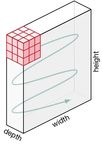
The kernel starts at the top-left corner of the input and moves right by the stride value, scanning horizontally. Once it reaches the edge, it returns to the left and shifts down by the stride to begin the next row. This top-to-bottom, left-to-right serpentine pattern continues until the entire input is covered.
 |
 |
| Kernel Movement (Static) | Kernel Movement (Animated) |
19.2.2 Activation Function (ReLU, Leaky ReLU, etc.)#
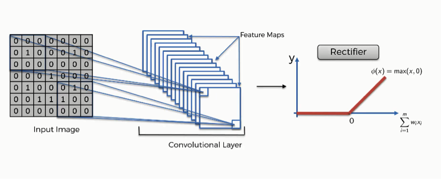
After each convolution, an activation function introduces non-linearity, allowing the network to learn complex patterns. The Rectified Linear Unit (ReLU) is the most widely used due to its simplicity and effectiveness in mitigating the vanishing gradient problem. ReLU outputs the input directly if it is positive; otherwise, it outputs zero.
 |
|
| Relu in CNN | How Relu Works |
The vanishing gradient problem occurs when gradients (used to update network weights during training) become very small, almost zero, especially in deep networks. This slows or stops learning because weights stop changing effectively. ReLU helps prevent this by allowing gradients to flow well for positive inputs.
In addition to introducing non-linearity, ReLU improves training efficiency by setting all negative values to zero. This creates sparsity in the network, meaning only the most important features (positive activations) are passed forward. This reduces complexity, helps the model focus on strong signals, and overall enables the CNN to learn faster and more effectively.
Other versions of ReLU, like Leaky ReLU and Parametric ReLU (PReLU), allow a small, non-zero output for negative input values instead of just zero. This helps avoid the problem of “dead neurons,” where some neurons stop learning completely.

19.2.3 Pooling Layers#
After applying convolution and activation (e.g., ReLU), a pooling layer (also called subsampling or downsampling) is used on the resulting feature map or activation map.
What is Pooling? A down-sampling operation that reduces the spatial dimensions (width and height) of the feature maps while keeping the most important information. This makes the network faster, uses less memory, and helps avoid overfitting.

Some of the most common types are:
Max Pooling: Selects the maximum value in each window of the feature map. It keeps the most important (strongest) features and helps detect edges or textures strongly.
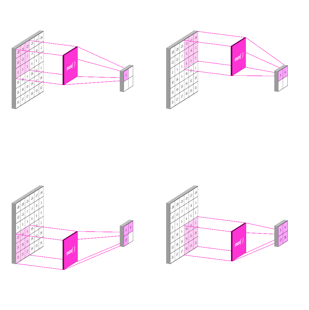
Average Pooling: Computes the average of all values in each window, providing smoother downsampling. This leads to smoother results, but may lose some important details. It is less commonly used in modern CNNs than max pooling.
Sum Pooling: Adds up all the values in the window. It behaves similarly to average pooling, but keeps the total strength of the signa
Pooling helps in achieving translation invariance, meaning the network becomes less sensitive to the exact position of features in the input.
Note: Translation invariance is an important concept in computer vision that helps neural networks recognize objects even if they shift slightly in an image. This means the model becomes less sensitive to small movements or changes in position. For example, if a feature like a cat’s ear or an edge moves a little to the left or right, the network can still recognize it. This is made possible by pooling layers, which summarize small regions of the activation maps—using operations like max or average—rather than keeping exact pixel locations. This allows the network to focus more on what feature is present, rather than where exactly it is. As a result, even when the appearance of an object changes slightly or it appears in a different location, the model can still identify it accurately. This makes translation invariance especially valuable for tasks like object detection and image classification.
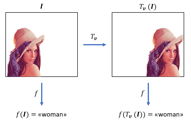
Figure: Let’s consider the images above. We can recognize a woman in both images even though the pixel values were shifted. An image classifier should predict the label “woman” for both images. In fact, the classifier output should not be influenced by the position of the target. Hence, the output of the classifier function is translation invariant. Ref:https://www.baeldung.com/cs/translation-invariance-equivariance.
19.2.4 Flattening and Fully Connected (Dense) Layer#
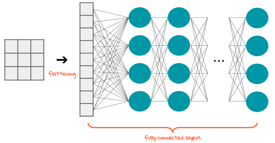
After several convolutional and pooling layers, the high-level features are flattened into a 1D vector and passed through one or more fully connected (dense) layers, just like in a traditional neural network. These layers perform the final classification or regression by combining all learned high-level features extracted by the convolutional layers. The last layer typically uses a softmax activation for classification or a linear activation for regression.
After several convolutional and pooling layers have extracted useful features, the output is flattened into a 1D vector—turning the multi-dimensional data into a simple list of numbers.
 |
 |
| Flattening | Flattening in CNN |
This vector is then passed to one or more fully connected (dense) layers, just like in a traditional neural network. These layers connect every input to every output, allowing the model to learn complex patterns by combining all the features. In the final layer:
Classification tasks often use: Softmax activation for multi-class output Sigmoid for binary output.
Regression tasks usually use: Linear activation to produce continuous values.

This part of the network is responsible for making the final prediction based on the high-level features extracted earlier.
19.3 Advantages of using CNNs Over Traditional Neural Networks.#
Traditional neural networks process input data in a flattened form, losing spatial structure and requiring an excessive number of parameters for high-dimensional data like images. CNNs overcome these limitations through:
Local Connectivity: Neurons in convolutional layers connect only to small regions of the input, reducing parameters while preserving spatial relationships.
Weight Sharing: The same filter is applied across the entire image (instead of having one weight per input feature (as in FFNNs), CNNs use one filter across many locations), drastically cutting down trainable weights and significantly reduces the number of parameters, allowing CNNs to scale to large input sizes like 224x224 images, which would be computationally intractable with fully connected layers.
Hierarchical Feature Learning: Early layers detect simple features (edges, textures), while deeper layers recognize complex patterns (shapes, objects).
This makes CNNs far more efficient for image-related tasks compared to fully connected networks.
19.4 Training CNNs#
The training process for CNNs is similar to that of traditional feedforward neural networks (FFNNs) and involves several key steps:
Feedforward pass: The input data passes through convolutional, activation, pooling, and fully connected layers to produce a prediction.
Loss computation: A loss function (such as cross-entropy for classification) measures the difference between the predicted output and the true label.
Backpropagation: Gradients of the loss with respect to all learnable parameters (filters, biases, weights) are calculated using the chain rule.
Parameter update: Optimizers like Stochastic Gradient Descent (SGD) or Adam adjust the parameters to minimize the loss.
To improve training and prevent overfitting, CNNs often include:
Dropout: Randomly disables a fraction of neurons during training to encourage the network to learn more robust features.
Batch Normalization: Normalizes layer inputs within each mini-batch to speed up training and improve stability.
Through many iterations of this process, the filters in the convolutional layers learn to extract increasingly abstract and useful features from the input data, enabling the model to make accurate predictions.
A simple CNN code snipets using Pytorch is given below:
import torch
import torch.nn as nn
import torch.nn.functional as F
import torch.optim as optim
from torchvision import datasets, transforms
from torch.utils.data import DataLoader

# Define the CNN model
class SimpleCNN(nn.Module):
    def __init__(self):
        super(SimpleCNN, self).__init__()
        self.conv1 = nn.Conv2d(1, 32, kernel_size=3)
        self.pool = nn.MaxPool2d(2, 2)
        self.dropout = nn.Dropout(0.25)  # dropout with 25% probability
        self.fc1 = nn.Linear(32 * 13 * 13, 10)

    def forward(self, x):
        x = self.pool(F.relu(self.conv1(x)))
        x = x.view(-1, 32 * 13 * 13)
        x = self.fc1(x)
        return x

# Device setup
device = torch.device("cuda" if torch.cuda.is_available() else "cpu")

# Transformations: ToTensor and Normalize
transform = transforms.Compose([
    transforms.ToTensor(),
    transforms.Normalize((0.1307,), (0.3081,))
])

# Load MNIST dataset (auto download if not present)
train_dataset = datasets.MNIST(root='./data', train=True, download=True, transform=transform)
test_dataset = datasets.MNIST(root='./data', train=False, download=True, transform=transform)

# Data loaders
train_loader = DataLoader(train_dataset, batch_size=64, shuffle=True)
test_loader = DataLoader(test_dataset, batch_size=1000, shuffle=False)

# Initialize model, loss, optimizer
model = SimpleCNN().to(device)
criterion = nn.CrossEntropyLoss()
optimizer = optim.Adam(model.parameters(), lr=0.001)

# Training loop example (1 epoch)
model.train()
for batch_idx, (data, target) in enumerate(train_loader):
    data, target = data.to(device), target.to(device)

    optimizer.zero_grad()
    output = model(data)
    loss = criterion(output, target)
    loss.backward()
    optimizer.step()

    if batch_idx % 100 == 0:
        print(f'Train Batch: {batch_idx}, Loss: {loss.item():.4f}')
---------------------------------------------------------------------------
ModuleNotFoundError                       Traceback (most recent call last)
Cell In[1], line 1
----> 1 import torch
      2 import torch.nn as nn
      3 import torch.nn.functional as F

ModuleNotFoundError: No module named 'torch'
#19.5 Transfer Learning in CNNs Transfer learning is a technique where a pretrained convolutional neural network (CNN), usually trained on a large dataset like ImageNet, is reused as the starting point for a new, related task. Instead of training a CNN from scratch (which requires a lot of data and computing resources), transfer learning leverages the knowledge the network has already learned—such as detecting edges, textures, and shapes.
There are two common ways to use transfer learning in CNNs:
Feature Extraction: The pretrained CNN’s convolutional base is used to extract features from new images. The fully connected layers at the end are replaced with new layers suited for the new task. The pretrained layers’ weights are usually frozen (not updated during training), and only the new classifier layers are trained.
Fine-tuning: After replacing the final layers, some or all of the pretrained convolutional layers are unfrozen and retrained (with a smaller learning rate). This allows the model to adapt more specifically to the new dataset while still using the valuable low-level features learned from the large original dataset.
Transfer learning is especially useful when you have limited labeled data for your target task, as it helps improve accuracy and speeds up training by starting from a pretrained model.
Summary of the Chapter#
CNNs are a powerful evolution of traditional neural networks tailored to work with spatial data like images. Their architecture—built on convolution, activation, and pooling layers—enables them to learn hierarchical, spatially-aware representations that general neural networks can’t.
A CNN consists of several key layers:
Convolutional layers: Extract features using learnable filters
Pooling layers: Reduce spatial dimensions (max pooling, average pooling)
Fully connected layers: Perform classification/Regression.
Activation functions: Introduce non-linearity (ReLU, softmax)
As we move forward, CNNs form the basis for advanced models in vision and even inspire architectures used in other domains such as NLP (e.g., CNN-based text classifiers).