Probability Distribution: From Single Events to Patterns#
So far, we have focused on individual events. In practice, data science is rarely about a single outcome.
Instead, we care about patterns across many observations.
A probability distribution describes how probability is spread across the possible values of a variable.
Some variables take countable values, such as the number of messages received today or the number of heads in ten coin flips. These follow discrete distributions.
Other variables vary smoothly, such as height, time, or temperature. These follow continuous distributions.
Mathematically: Probability Distributions
A random variable \(X\) assigns numerical values to outcomes in the sample space.
Discrete random variables take countable values.
Their probabilities are given by \(P(X = x)\) and satisfy\(\sum_x P(X = x) = 1\).
Continuous random variables take values on a continuum.
They are described by a probability density function \(f(x)\) such that\(\int_{-\infty}^{\infty} f(x)\,dx = 1\).
For continuous variables, \(P(X = c) = 0\) for any single value \(c\).

Difference Between Discrete and Continuous Variables. Source: GeeksforGeeks.
Distributions allow us to reason about averages, variability, typical behavior, and rare extremes.
They turn uncertainty into structure, which is why they are central to data science.
Small Python Simulation
Discrete vs continuous samples.
import numpy as np
import matplotlib.pyplot as plt

np.random.seed(0)
n = 10_000

# Discrete: number of successes
X_discrete = np.random.binomial(n=10, p=0.5, size=n)

# Continuous: measurement noise
X_continuous = np.random.normal(loc=0, scale=1, size=n)

plt.figure()
plt.hist(X_discrete, bins=np.arange(-0.5, 11.5, 1), density=True)
plt.title("Discrete Distribution (Binomial)")
plt.xlabel("Value")
plt.ylabel("Probability")
plt.show()

plt.figure()
plt.hist(X_continuous, bins=40, density=True)
plt.title("Continuous Distribution (Normal)")
plt.xlabel("Value")
plt.ylabel("Density")
plt.show()
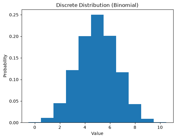
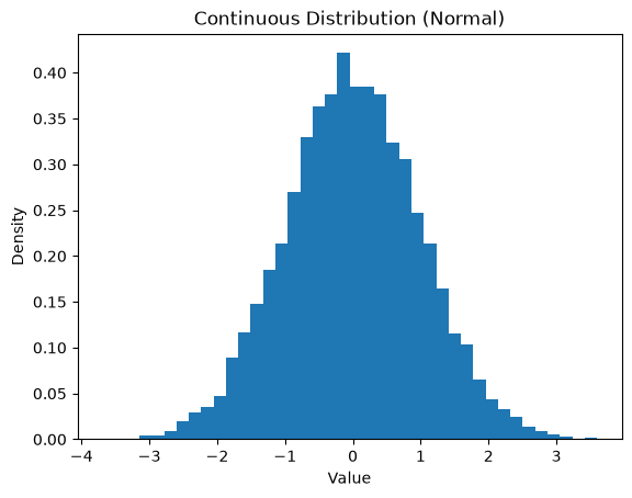
Notice: Discrete distributions have separate bars and Continuous distributions form smooth shapes. Both describe uncertainty, but in different ways.
Common Distributions You Will See Everywhere#
In data science, we do not just ask what happened.
We ask how values behave across many observations.
A probability distribution describes the data-generating process behind what we observe.
Probability distributions are broadly divided into discrete and continuous distributions.
(1) Discrete distributions model outcomes that take countable values:
Bernoulli Distribution
Binomial Distribution
Poisson Distribution
Zero-Inflated Poisson Distribution
(2) Continuous distributions model outcomes that vary smoothly over an interval:
Uniform Distribution
Normal (Gaussian) Distribution
Many more
Why This Matters#
Different datasets come from different processes:
clicks vs. no-clicks
event counts per hour
measurements with noise
Understanding how your data is distributed tells you a lot about how the data was generated.
Distribution Choice and Analysis
The nature of a distribution affects:
which statistical assumptions are reasonable
which models are appropriate
which evaluation metrics make sense
Choosing the wrong distribution can lead to incorrect conclusions, even when the computations are correct.