Central Limit Theorem (Why Normal Appears Everywhere)#
In data science, we repeatedly see the Normal distribution, even when the original data is not normal. The reason is the Central Limit Theorem (CLT).
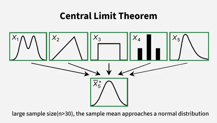
CLT Theorem: Regardless of the original distribution, the distribution of sample means approaches a Normal distribution as sample size increases.
Mathematically: Central Limit Theorem (Informal)
Let \(X_1, X_2, \dots, X_n\) be independent random variables with the same mean \(\mu\) and finite variance.
As \(n\) becomes large, the distribution of the sample mean
\(\bar{X} = \frac{1}{n}\sum_{i=1}^n X_i\)
approaches a Normal distribution, regardless of the original distribution of the data.
Intuition:
Individual data points can be messy, skewed, or discrete
Averages of many observations become predictable
Noise cancels out, and structure emerges
This is why:
averages of clicks
average model errors
average measurements
often behave normally, even if the raw data does not.
Central Limit Theorem Visual Overview#
 Bernoulli distribution (Slideserve) |
 Bernoulli PMF/Outcome illustration (Medium) |
 Bernoulli PMF/Outcome illustration (Medium) |
These figures illustrate why sample means tend to follow a Normal distribution, even when the original data is not Normal.
Python Simulation: CLT in Action
We will start with data that is not normal (Uniform), then look at averages.
import numpy as np
import matplotlib.pyplot as plt

np.random.seed(0)

n_samples = 20_000

# Step 1: raw data (uniform, not normal)
raw = np.random.uniform(0, 1, size=n_samples)

# Step 2: averages of multiple samples
k = 30
averages = np.mean(
    np.random.uniform(0, 1, size=(n_samples, k)),
    axis=1
)

plt.figure()
plt.hist(raw, bins=40, density=True)
plt.title("Raw Data: Uniform(0,1)")
plt.xlabel("Value")
plt.ylabel("Density")
plt.show()

plt.figure()
plt.hist(averages, bins=40, density=True)
plt.title("Averages of 30 Uniform Samples (CLT)")
plt.xlabel("Value")
plt.ylabel("Density")
plt.show()
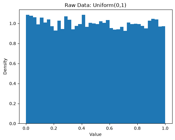

Notice: Even when the raw data is not bell-shaped, the averages form a bell-shaped curve. This happens without assuming normal data; this is the Central Limit Theorem at work.
Why CLT Matters in Data Science#
The Central Limit Theorem explains why we can:
use Normal-based confidence intervals
apply z-tests and t-tests
model average error with Gaussian assumptions
trust metrics based on means
Data Science Insight
Many statistical tools assume normality of averages, not raw data.
This assumption is justified by the Central Limit Theorem.