(II) Measures of Shape: Skewness, Modality, and Distribution Behavior#
Understanding the center is not enough.
Two datasets can have:
The same mean
The same median
The same variance
And still look completely different. That’s why we must understand shape.
(II.a) Skewness: Which Direction Is the Tail?#
Skewness describes the asymmetry of a distribution. It tells us whether one tail is longer than the other.
Three Main Cases#
Symmetric (Zero-Skewed) Distribution
Mean ≈ Median
Tails are balanced
Example: Exam scores in a well-calibrated course
Right-Skewed (Positively Skewed)
Long tail to the right
Mean > Median
Extreme large values pull the mean upward
Left-Skewed (Negatively Skewed)
Long tail to the left
Mean < Median
Extreme small values pull the mean downward
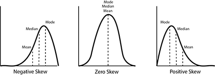
Figure: Comparison of symmetric, right-skewed, and left-skewed distributions, showing the relative positions of mean, median, and mode. Source: Miro.Medium.
Example: Skewness in Real Life
Startup salaries: A few extremely high values create a long right tail → Right skew (Mean > Median)
Easy exam scores: A few very low values create a long left tail → Left skew (Mean < Median)
Rule: Skewness always points toward the long tail.
Why Skewness Matters?#
Skewness helps us understand how data is distributed. When data is highly skewed, a few extreme values can pull the mean toward the long tail, making it less representative of most observations. In these cases, the median often gives a better idea of a typical value, and knowing the skewness helps us interpret averages more correctly.
(II.b) Modality: How Many Peaks?#
Modality describes the number of peaks in a distribution.
It helps reveal whether the data comes from one group or multiple distinct groups.
Types of Modality#
Unimodal
One peak
One dominant group
Bimodal
Two peaks
Two distinct subgroups
Multimodal
More than two peaks
Multiple underlying processes

Figure: Examples of distribution modality: unimodal, bimodal, uniform, and multimodal; showing how the number of peaks reveals the underlying structure of the data. Source:Stack Overflow.
Modality helps us understand whether the data comes from one group or multiple distinct groups.
Why Modality Matters#
Modality helps us determine whether data represents:
One homogeneous group
Multiple distinct groups
Different underlying behaviors
Ignoring modality can hide important patterns within the data.
Quick Rule: Each peak often represents a different subgroup in
Example: Remote vs In-Office Work Hours#
You measure daily working hours:
Remote workers: 7–8 hours
In-office workers: 9–10 hours
The histogram shows two peaks, one for each group.
Although the overall mean may be around 8.5 hours, there is no single “typical” worker because the data contains two distinct populations.
This is an example of a bimodal distribution.
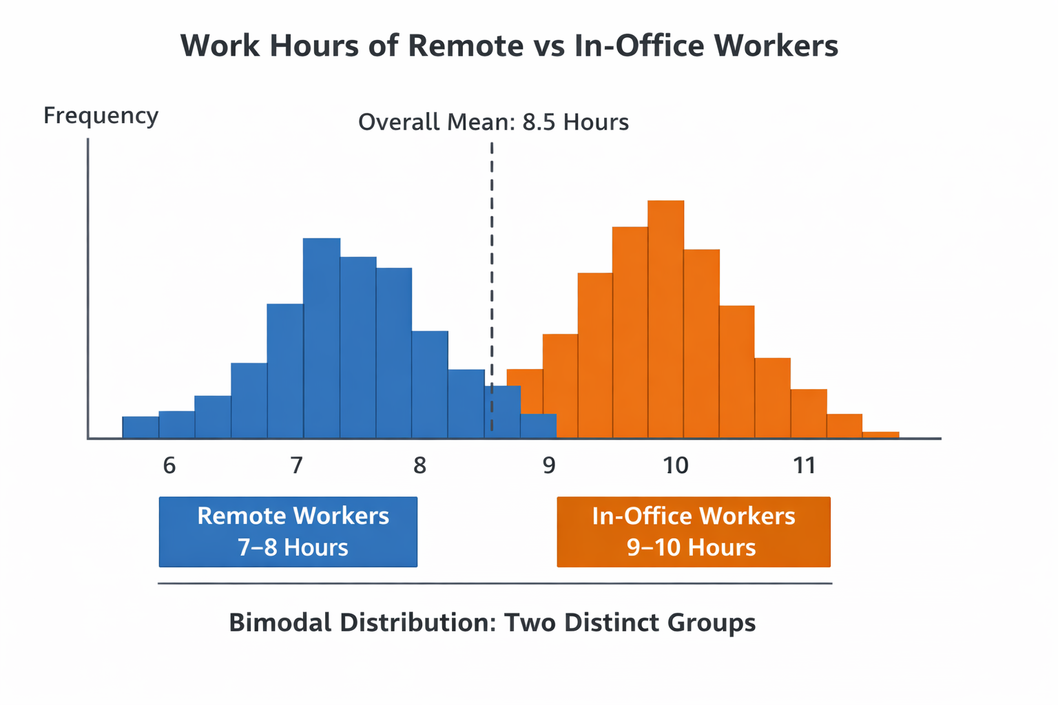
Figure: A bimodal distribution showing two distinct peaks, representing two underlying groups.
Beyond skewness and modality, we also look at:
Outliers#
Outliers are data points that are far from most other values.
They can:
Indicate data entry errors
Represent rare but important events
Suggest a different underlying data-generating process
Important: Not all outliers should be removed; they may contain valuable information.