Inspecting Data: First Contact

Inspecting Data: First Contact#

The moment a DataFrame loads, the first questions are never about modeling; they are always about shape:

How many rows?
How many columns?
What are the datatypes?
Are there missing values? -Does it look reasonable?

Pandas has a small vocabulary for these basic operations.

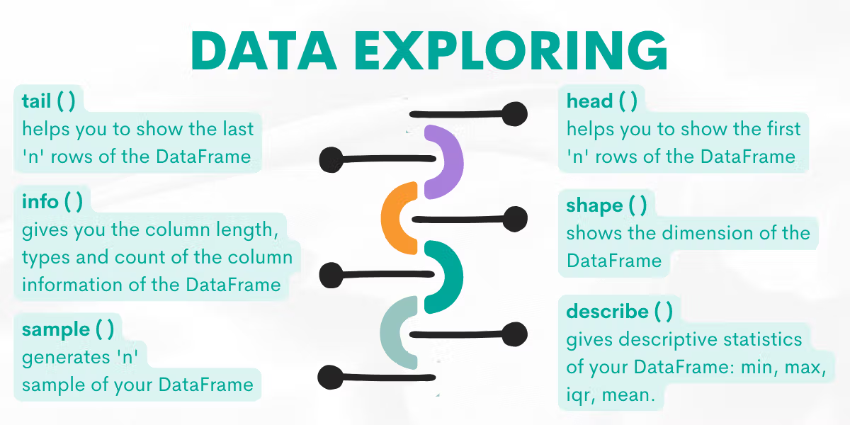
Pandas Basic Operations#

After reading tabular data as a DataFrame, you would need to have a glimpse of the data. Pandas makes it easy to explore and manipulate. A good first step is to inspect the dataset by previewing how many rows and columns it has, what the column names are, checking dimensions, or reviewing summary information such as data types and statistics. Pandas provides convenient methods for this.

##Viewing/Exploring Data

Command	Description	Default Behavior
`df.head()`	Displays the first rows of the DataFrame. Useful for quickly previewing the dataset.	Shows 5 rows
`df.tail()`	Displays the last rows of the DataFrame. Handy for checking the dataset’s ending records.	Shows 5 rows
`df.shape`	Returns a tuple `(rows, columns)` representing the dimensions of the DataFrame.	N/A
`df.info()`	Shows column names, data types, memory usage, and count of non-null values.	N/A
`df.dtypes`	Returns the data type of each column in the DataFrame.	N/A
`df.describe()`	Provides summary statistics (mean, std, min, max, quartiles) for numeric columns.	Includes numeric columns by default

These lines form the “hello world” of any data-driven project.

Even in professional settings, someone uploads a CSV to Slack, someone loads it into Pandas, and the first message back is almost always:

“Wait, why is year stored as string?”

or

“We have 800k rows. Expected 500k. Did we duplicate something?”

Learning to inspect before analyzing is a habit that prevents embarrassment later.

import pandas as pd

data = {
    'Name': ['Alice', 'Bob', 'Charlie'],
    'Age': [24, 30, 28],
    'Salary': [50000, 60000, 55000]
}
df = pd.DataFrame(data)

print("head")
print(df.head())
print("shape")
print(df.shape)
print("info")
print(df.info)

head
      Name  Age  Salary
0    Alice   24   50000
1      Bob   30   60000
2  Charlie   28   55000
shape
(3, 3)
info
<bound method DataFrame.info of       Name  Age  Salary
0    Alice   24   50000
1      Bob   30   60000
2  Charlie   28   55000>

Selecting and Indexing Data#

After inspecting the structure of a DataFrame, the next step is often to select specific rows and columns (specific parts of the data). Pandas provides several approaches depending on whether you want to select columns, rows, or filter data based on conditions. It lets you choose columns, rows, or both using labels (loc), integer positions (iloc), or conditions.

1. Selecting Columns#

Command	Description
`df['col']`	Selects a single column as a Series.
`df[['col1','col2']]`	Selects multiple columns as a new DataFrame.

2. Selecting Rows#

Command	Description
`df.loc[row_label]`	Select row(s) by label (index name).
`df.iloc[row_index]`	Select row(s) by integer position.
`df.loc[0, 'col']`	Select a specific value by row & column.

3. Conditional Selection (Filtering)#

Command	Description
`df[df['col'] > 50]`	Returns rows where condition is True.
`df[(df['A'] > 50) & (df['B'] < 100)]`	Combine conditions with `&` (and), `	` (or).

Follow is an example:

import pandas as pd

data = {
    'Name': ['Alice', 'Bob', 'Charlie'],
    'Age': [24, 30, 28],
    'City': ['New York', 'Los Angeles', 'Chicago']
}

df = pd.DataFrame(data)
print(df)

# Now, to access the columns: Select columns
df['Age']
df[['Name', 'City']]

# Select rows
df.iloc[0]        # First row
df.iloc[1:3]      # Rows 1–2
df.loc[0, 'Name'] # Specific cell

# Conditional selection
df[df['Age'] > 30]
df[(df['Age'] > 30) & (df['City'] == 'Chicago')]

      Name  Age         City
  Alice   24     New York
    Bob   30  Los Angeles
Charlie   28      Chicago

	Name	Age	City

Adding a new column to DataFrame#

A new column can be added to a pandas DataFrame by assigning a value, list, or Series to a new column name. If the assigned data is a list or Series, its length must match the number of rows in the DataFrame. You can also assign a single value, which will be applied to all rows.

import pandas as pd

df = pd.DataFrame({
    "Name": ["Alice", "Bob", "Charlie"],
    "Math": [90, 85, 95]
})
print(df)

# Add a new column with a list
df["English"] = [88, 92, 80]

print(df)

# Add a new column with a single value
df["Pass"] = True

print(df)

      Name  Math
  Alice    90
    Bob    85
Charlie    95
      Name  Math  English
  Alice    90       88
    Bob    85       92
Charlie    95       80
      Name  Math  English  Pass
  Alice    90       88  True
    Bob    85       92  True
Charlie    95       80  True

Arithmetic Operations and Functions in Pandas#

So far we explored how to inspect and select data in Pandas. Once you have access to the right rows and columns, the next step is to perform calculations and apply functions. Pandas makes this process very intuitive by allowing you to apply arithmetic directly to DataFrames or Series, and by offering tools like apply(), map(), and applymap() for more flexibility.

Arithmetic Operations on Columns#

You can directly apply mathematical operations to Pandas Series or DataFrame columns. Operations are vectorized, meaning they are applied element-wise across the column.

In below example, you can notice how the operations are automatically applied to each row.

import pandas as pd

data = {
    'Name': ['Alice', 'Bob', 'Charlie'],
    'Age': [24, 30, 28],
    'Salary': [50000, 60000, 55000]
}
df = pd.DataFrame(data)
print(df)

# Increase all salaries by 10%
df['Salary'] = df['Salary'] * 1.10

# Add 5 years to everyone’s age
df['Age'] = df['Age'] + 5
print(df)

      Name  Age  Salary
  Alice   24   50000
    Bob   30   60000
Charlie   28   55000
      Name  Age   Salary
  Alice   29  55000.0
    Bob   35  66000.0
Charlie   33  60500.0

Arithmetic Between Columns#

You can also perform arithmetic between two or more columns to create new features.

# Create a new column 'Income_per_Age'
df['Income_per_Age'] = df['Salary'] / df['Age']
print(df)

      Name  Age   Salary  Income_per_Age
  Alice   29  55000.0     1896.551724
    Bob   35  66000.0     1885.714286
Charlie   33  60500.0     1833.333333

Applying Built-in Pandas/Numpy Functions#

Pandas integrates with NumPy functions, allowing you to apply common statistics directly.

import numpy as np

# Calculate average salary
print(df['Salary'].mean())

# Standard deviation of Age
print(df['Age'].std())

# Apply numpy square root
print(np.sqrt(df['Age']))

0
0550504633038935
  5.385165
  5.916080
  5.744563
Name: Age, dtype: float64

Applying Functions with apply()#

Sometimes you need custom transformations. The apply() method lets you apply a function to an entire column (Series) or to each row/column in a DataFrame.

# Apply to a Series
df['Age_squared'] = df['Age'].apply(lambda x: x**2)

# Apply to DataFrame across rows
df['Total'] = df[['Age','Salary']].apply(lambda row: row['Age'] + row['Salary'], axis=1)
print(df)

      Name  Age   Salary  Income_per_Age  Age_squared    Total
  Alice   29  55000.0     1896.551724          841  55029.0
    Bob   35  66000.0     1885.714286         1225  66035.0
Charlie   33  60500.0     1833.333333         1089  60533.0