(I). Measures of Location: Where Is the Center?#
If you plotted your data on a number line, where would the “center” be?
At first, this seems like a simple question, but mathematically, the answer depends on how we define what it means to be “close” to the data.
There are two main ways to define closeness:
Absolute distance → leads to the median
Squared distance → leads to the mean
Because these definitions are different, they produce different notions of “center.”
(I.a) The Arithmetic Mean#
The arithmetic mean is what most people call the “average.”
The mean minimizes the sum of squared distances:
That squared term is important. Squaring makes large distances dramatically more influential.
The mean is very sensitive to extreme values (outliers).
Example:#
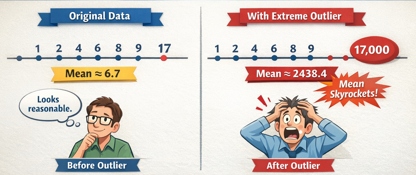
Figure: Replacing a single value (17 → 17000) drastically increases the mean, showing why the mean is not robust to extreme values.
The mean works well when:
Data is roughly symmetric
Outliers are meaningful (not errors)
Total magnitude matters
Example:
Average temperature
Average revenue
Average exam score in a balanced class
(I.b) The Median#
The median is the middle value after sorting the data.
If the dataset has an odd number of values → pick the middle one
If even → take the average of the two middle values
The median minimizes the sum of absolute distances:
Unlike squaring, absolute distance does not amplify extremes. So the median is robust to outliers.
Example (Income Data)#
Income distributions are usually right-skewed:
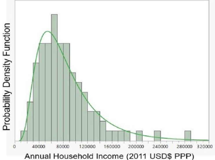
Figure: Most people earn moderate incomes. A few people earn extremely high incomes
Because of this:
Mean income becomes much larger
Median income stays closer to what most people earn
So the median gives a more realistic “typical value.”
When Mean and Median Differ?#
The difference between them tells us about skewness:
Symmetric distribution → Mean ≈ Median
Right-skewed distribution → Mean > Median
Left-skewed distribution → Mean < Median
Remember: The mean reacts to the extreme values and the median resists it.
(We will revisit this idea later in the chapter.)
Weighted Mean: When All Data Points Are Not Equal#
Sometimes, observations should not contribute equally.
Example: Averaging housing prices across states.
If you ignore population size:
A small state influences the average as much as a large state.
This produces misleading conclusions.
In such cases, we use a weighted mean:
Where:
\(w_i\) = weight (population, sample size, frequency)
\(x_i\) = observation
Failing to weight appropriately can significantly distort interpretation.