Step 1: Define the Hypotheses#
Every hypothesis test begins with two competing statements.
Null Hypothesis (H₀)#
The “nothing changed” claim.
It represents the default world — no effect, no difference, no improvement.
Example:
The new recommendation system does NOT change average order value.
Mathematically: $\(H₀: \mu_{\text{new}} = \mu_{\text{old}}\)$
Alternative Hypothesis (H₁ or Ha)#
The claim we are testing for.
Example:
The new system increases average order value.
Mathematically: $\(H₁: \mu_{\text{new}} > \mu_{\text{old}}\)$
Why Assume the Null Is True?#
Because science is cautious.
We don’t claim something works just because numbers look different.
We require strong evidence.
Think of it like this:
If data fits normal random variation → keep the null
If data looks extremely unlikely → reject the null
Step 2: Understand Random Variation#
Even if nothing changes, data still fluctuates.
Example:
Daily average order values might look like: 24.1, 23.8, 24.6, 24.0, 25.0, 23.9 …
Variation is natural.
So when we see $25.30, we must ask:
Is this within normal variation?
Or unusually large?
To answer this, we calculate a probability.
Step 3: Choose a Significance Level (α)#
Before we look at the data too deeply, we decide:
How much risk of a false alarm are we willing to accept?
This risk is the significance level, written as α. Common choice: α = 0.05
Meaning:
We accept a 5% chance of rejecting the null hypothesis even when it is actually true (this is called a Type I error).
You can think of α like a strictness setting:
Smaller α (like 0.01) → harder to reject H₀
Larger α (like 0.10) → easier to reject H₀
Step 4: Two Ways to Make the Same Decision#
There are two equivalent ways to decide whether to reject the null hypothesis:
The critical value (rejection region) approach
The p-value approach
Both use the same elements:
significance level (α)
sampling distribution
observed test statistic
They differ only in how the decision is evaluated.
Step 4A: Critical Value and Rejection Region#
The critical value approach defines a decision boundary.
Critical Value#
A critical value is the cutoff separating likely from unlikely outcomes under the null hypothesis. If the test statistic crosses this boundary, the result is statistically significant. It depends on:
significance level (α)
sampling distribution (z, t, etc.)
one-tailed vs two-tailed test
Rejection Region#
The rejection region contains test statistic values considered too unlikely if H₀ is true. These lie in the extreme tails of the sampling distribution.
Decision rule:
inside rejection region → reject H₀
outside rejection region → fail to reject H₀
Total probability of rejection region = α.
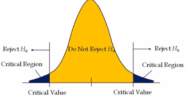
One-Tailed vs Two-Tailed Tests#
The rejection region depends on the research question.
One-tailed test: interest in one direction only → all α in one tail.
Two-tailed test: interest in any difference → α split across both tails.
Example (α = 0.05):
one-tailed → 0.05 in one tail
two-tailed → 0.025 in each tail

Step 4B: p-Value Approach#
The p-value measures how extreme the observed result is under the null hypothesis.
Decision rule:
p-value ≤ α → reject H₀
p-value > α → fail to reject H₀
How the Two Methods Are Connected#
Both approaches compare probability to α:
critical value method → compare statistic to boundary
p-value method → compare probability to α
They always lead to the same decision.
Example#
Two-tailed test
α = 0.05
critical values = ±1.96
observed statistic = 2.30
Critical value method → 2.30 > 1.96 → reject H₀
p-value method → p = 0.021 < 0.05 → reject H₀
Hypothesis testing asks whether the observed result is too unlikely under the null hypothesis to be explained by chance alone.
Step 5: Compute the Test Statistic#
After defining the decision rule, the next step is to measure how extreme the observed data actually is.
We do this by computing a test statistic, a standardized numerical summary that compares the sample result to what we would expect if the null hypothesis were true. In simple terms, the test statistic answers:
How far is the observed result from what we would expect under H₀?
The choice of test statistic depends on the data and research question. Common examples include:
z-statistic → when population variability is known
t-statistic → when population variability is unknown (most common)
χ² statistic → categorical data
F statistic → comparing multiple group means (ANOVA)
The test statistic places the observed result on the sampling distribution. Once computed, it is compared to the decision rule defined in Step 4 (critical value or p-value). This comparison determines whether the result is statistically significant.
To measure how extreme the observed data is under the null hypothesis, we compute a test statistic.
The type of statistic depends on the test being used.
z-test → population variance known
t-test → population variance unknown (most common)
chi-square → categorical data
ANOVA → comparing multiple groups
For comparing means in data science, we most often use a t-test.
import numpy as np
import matplotlib.pyplot as plt
from scipy.stats import norm, t

x = np.linspace(-4,4,500)

plt.figure(figsize=(8,5))
plt.plot(x, norm.pdf(x), label="Z distribution (normal)")
plt.plot(x, t.pdf(x, df=5), label="t distribution (df=5)")
plt.plot(x, t.pdf(x, df=30), label="t distribution (df=30)")
plt.title("Z vs t Distribution")
plt.xlabel("Value")
plt.ylabel("Density")
plt.legend()
plt.show()
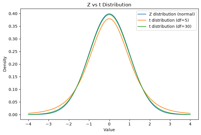
Notice:
Small sample → thicker tails → more uncertainty
Large sample → t looks like normal
As sample size increases, t-test becomes similar to z-test.