Types of Regression#
As we move from simple problems to more complex ones, different types of regression models are used depending on the nature of the data and the relationship.
1. Simple Linear Regression#
The simplest form of regression is linear regression with one variable, where we assume a straight-line relationship between input and output.
we model the relationship between one feature and the target using a straight line. Example: Predicting salary based on years of experience
One input variable
Assumes a linear relationship
Easy to interpret
The model is written as:
Where:
\(y\) is the predicted value
\(x\) is the input feature
\(m\) is the slope (how much \(y\) changes with \(x\))
\(b\) is the intercept (value of \(y\) when \(x=0\))
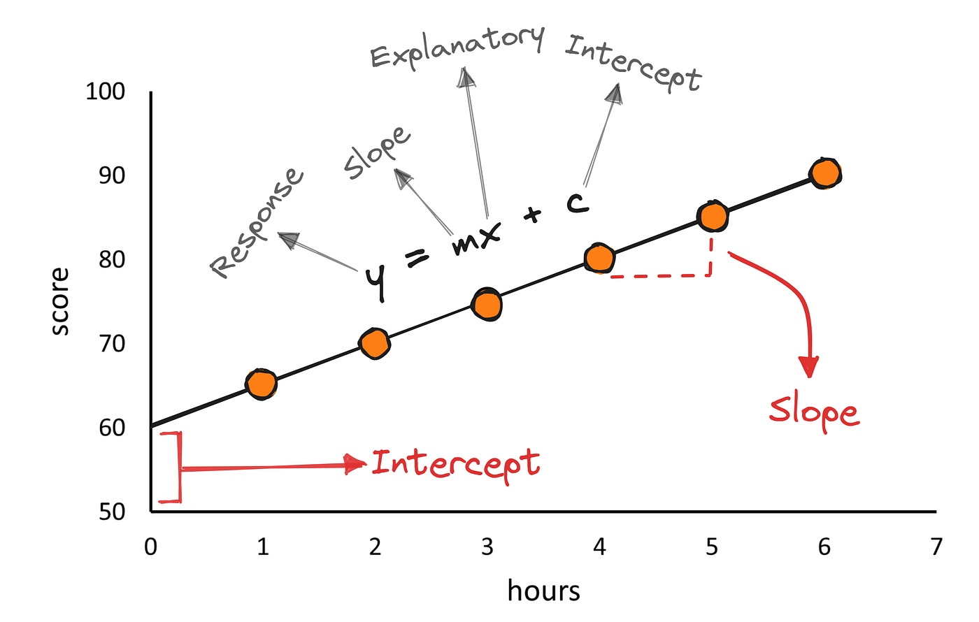
A Simple View of Linear Regression. Source:Medium.com
Intuition#
Think of this as fitting the “best possible straight line” through your data points. The model tries to capture the overall trend in the data.
For example:
If house size increases, price usually increases → positive slope
If study hours increase, exam score increases → positive slope
Key Insight: The model does not try to pass through every point. Instead, it minimizes the overall error across all points.
2. Multiple Linear Regression#
In reality, most outcomes depend on multiple factors, a single feature is rarely sufficient. Multiple linear regression extends the idea of a straight line to multiple dimensions.
Multiple input variables
Each feature contributes to the prediction
Helps capture more realistic scenarios
Example: Predicting house price depends on:
Size
Number of bedrooms
Location
Age of the property
This leads to multiple linear regression, where we use several features:
Where:
\(n\) is the degree of polynomial
\(b_0\) is the intercept
\(b_1, b_2, \dots, b_n\) are coefficients
Each \(x_i\) is a feature
Each feature contributes independently to the prediction.
Interpretation#
One of the most powerful aspects of multiple regression is interpretation:
\(b_1\): effect of \(x_1\) while keeping all other variables constant
\(b_2\): effect of \(x_2\), and so on
This allows us to answer questions like:
“How much does price increase per extra bedroom, holding size constant?”
Important Note#
Features should not be highly correlated with each other (multicollinearity), as it can make interpretation unstable.
3. Non-Linear Relationships and Polynomial Regression#
Not all relationships are linear. Sometimes the data curves Polynomial regression allows the model to fit curves instead of straight lines.
Captures non-linear patterns
Still based on linear modeling techniques
Risk of overfitting if degree is too high
Example:
Growth may accelerate over time
Costs may increase at an increasing rate
To handle this, we use polynomial regression:

A Simple View of Polynomial Regression. Source: Statisticalaid.com
Even though the curve looks non-linear, the model is still linear in parameters, which allows us to train it using the same techniques as linear regression.
Tradeoff#
Low degree → underfitting
High degree → overfitting
Choosing the right degree is critical.
Python Implementation#
In practice, regression is often implemented using libraries such as:
### Basic Linear Regression

```python
from sklearn.linear_model import LinearRegression
from sklearn.model_selection import train_test_split

# split data
X_train, X_test, y_train, y_test = train_test_split(X, y, test_size=0.2)

# train model
model = LinearRegression()
model.fit(X_train, y_train)

# predictions
predictions = model.predict(X_test)


### Basic Polynomial Regression

from sklearn.preprocessing import PolynomialFeatures

poly = PolynomialFeatures(degree=2)
X_poly = poly.fit_transform(X)

model = LinearRegression()
model.fit(X_poly, y)