import networkx as nx
import matplotlib.pyplot as plt
import numpy as np

Graph Featurization

Raw graph structure alone is not always enough for machine learning. Featurization converts graph structure and node/edge properties into numeric vectors that models can consume.

Why Featurization?

Graphs are inherently relational, but most ML models expect fixed-size numeric inputs. Featurization bridges this gap.

Types of Graph Features

There are four main types:

Type	What it captures	Examples
1. Graph-level features	Properties of the whole graph	Diameter, density, spectral features
2. Edge features	Properties of connections	Weight, transaction amount, timestamp
3. Node features	Properties of individual nodes	Age, degree, label
Structural features	Topological role of a node	Centrality, clustering coefficient, motif count

In Graph Neural Networks, the model learns to aggregate these features across multi-hop neighborhoods automatically.

1. Graph-Level Features (Global View)

Describe the entire graph as a whole.

What they capture:

• Overall connectivity

• Global structure

• Network complexity

Common Features:

• Diameter → longest shortest path in the graph

• Average path length → average distance between nodes

• Density → how many edges exist vs possible edges

• Modularity → strength of community structure

Example:

• Social network: High density → many people are connected; Low diameter → information spreads quickly.

• Used in: Graph classification (e.g., molecule type, network type)

2. Edge-Level Features (Relationship View)

Describe connections between two nodes.

What they capture:

• Strength or nature of relationships

• Likelihood of future connections

Common Features:

• Weight → distance, cost, interaction frequency

• Common neighbors → shared connections

• Jaccard similarity → similarity between neighborhoods

• Edge betweenness → importance of an edge

Example:

• E-commerce:

  • Edge = user → product

  • Weight = number of purchases

• Social network:

  • Two users with many common friends → high similarity

Used in: Link prediction, Recommendation systems, Fraud detection.

3. Node-Level Features (Local View — Focus)

Describe individual nodes. There are two ways - via “Degree” and via “Centrality”

(a) Degree:

Number of connections a node has
Types:

• In-degree → incoming edges

• Out-degree → outgoing edges

Example:

• Twitter:

  • High in-degree → many followers

  • High out-degree → follows many people

Interpretation:High degree → more connected → potentially more influence

(b) Centrality (Covered Next Section)

Centrality measures capture node importance in the network.

• Degree Centrality: Measures importance based on the number of direct connections a node has.

• Closeness Centrality: Measures how quickly a node can reach all other nodes in the network.

• Betweenness Centrality: Measures how often a node lies on the shortest paths between other nodes (bridge nodes).

• Eigenvector Centrality: Measures importance by considering not just connections, but how important those neighbors are.

4. Structural Features (Topological Role)

Describe how a node is positioned in the overall structure.

What they capture:

• Local neighborhood patterns

• Role of node in graph structure

Common Features:

• Clustering coefficient → how connected neighbors are

• Triangle count → number of triangles a node participates in

• Motifs → recurring subgraph patterns

Example:

• Social network:High clustering → tight friend group

• Fraud detection: Unusual patterns → suspicious behavior

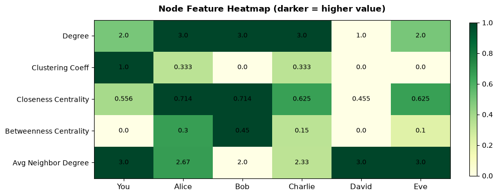
# ── Build a feature table for each node ─────────────────────────────────────
features = {}
for node in G.nodes():
    deg   = G.degree(node)
    cc    = nx.clustering(G, node)
    close = nx.closeness_centrality(G, node)
    betw  = nx.betweenness_centrality(G)[node]
    neigh_degrees = [G.degree(nb) for nb in G.neighbors(node)]
    avg_nb_deg = np.mean(neigh_degrees) if neigh_degrees else 0

    features[node] = {
        'Degree':                      deg,
        'Clustering Coeff':            round(cc,   3),
        'Closeness Centrality':        round(close,3),
        'Betweenness Centrality':      round(betw, 3),
        'Avg Neighbor Degree':         round(avg_nb_deg, 2),
    }

df_features = pd.DataFrame(features).T
df_features.index.name = 'Node'
print("=== Node Feature Matrix (structural features) ===")
print(df_features.to_string())

# Heatmap
fig, ax = plt.subplots(figsize=(10, 4))
data_norm = df_features.apply(lambda col: (col - col.min()) / (col.max() - col.min() + 1e-9))
im = ax.imshow(data_norm.T.values, cmap='YlGn', aspect='auto', vmin=0, vmax=1)
ax.set_xticks(range(len(df_features)))
ax.set_yticks(range(len(df_features.columns)))
ax.set_xticklabels(df_features.index, fontsize=11)
ax.set_yticklabels(df_features.columns, fontsize=10)
for i, col in enumerate(df_features.columns):
    for j, node in enumerate(df_features.index):
        ax.text(j, i, df_features.loc[node, col], ha='center', va='center', fontsize=9)
ax.set_title('Node Feature Heatmap (darker = higher value)', fontsize=12, fontweight='bold', pad=12)
plt.colorbar(im, ax=ax, fraction=0.02)
plt.tight_layout()
plt.show()

=== Node Feature Matrix (structural features) ===
         Degree  Clustering Coeff  Closeness Centrality  Betweenness Centrality  Avg Neighbor Degree
Node                                                                                                
You         2.0             1.000                 0.556                    0.00                 3.00
Alice       3.0             0.333                 0.714                    0.30                 2.67
Bob         3.0             0.000                 0.714                    0.45                 2.00
Charlie     3.0             0.333                 0.625                    0.15                 2.33
David       1.0             0.000                 0.455                    0.00                 3.00
Eve         2.0             0.000                 0.625                    0.10                 3.00