2. Feature Transformation

Feature transformation refers to modifying existing features to improve their scale, distribution, or representation so that machine learning models can learn patterns more effectively.

Common transformation techniques include:

• Scaling and Normalization

• Standardization

• Log Transformation

• Encoding Categorical Variables

• Discretization (Binning)

• Text Feature Extraction (Later Chapter)

2a. Scaling and Normalization

Scaling adjusts the range of numerical values so that features are comparable.

Example:

Feature	Range
Age	18 – 60
Income	20,000 – 200,000

Because income has a much larger range, some models may give it more influence.

Min-Max Normalization

This method rescales values to the 0–1 range.

\[ x' = \frac{x - min(x)}{max(x) - min(x)} \]

Example python code:

from sklearn.preprocessing import MinMaxScaler

scaler = MinMaxScaler()
df_scaled = scaler.fit_transform(df[["income"]])

Standardization

Standardization transforms values so that they have mean = 0 and standard deviation = 1

Formula:

\[ z = \frac{x - 𝜇}{σ} \]

Where:

• μ = mean

• σ = standard deviation

Example python code:

from sklearn.preprocessing import StandardScaler

scaler = StandardScaler()
df_standardized = scaler.fit_transform(df[["income"]])

Standardization is commonly used in algorithms such as:

• Logistic Regression

• Support Vector Machines

• K-Means Clustering

2b. Log Transformation

Log transformation is used when data is highly skewed or contains very large values.
It helps reduce the influence of extreme values and makes the distribution more balanced.

Example Data

Income
30000
40000
50000
900000

Applying a log transformation compresses large values.

\[ x' = \log(x) \]

This transformation is commonly used for variables such as:

• income

• population

• sales

• transaction amounts

import pandas as pd
import numpy as np
import matplotlib.pyplot as plt

# Example dataset
df = pd.DataFrame({
    "income": [30000, 40000, 50000, 900000]
})

# Apply log transformation
df["log_income"] = np.log(df["income"])

df

	income	log_income
0	30000	10.308953
1	40000	10.596635
2	50000	10.819778
3	900000	13.710150

# another example
import numpy as np
import matplotlib.pyplot as plt

# Generate skewed income data
np.random.seed(42)
income = np.random.lognormal(mean=10, sigma=1, size=1000)

# Log transform
log_income = np.log(income)

plt.figure(figsize=(12,5))

plt.subplot(1,2,1)
plt.hist(income, bins=40)
plt.title("Original Income Distribution (Right-Skewed)")
plt.xlabel("Income")
plt.ylabel("Frequency")

plt.subplot(1,2,2)
plt.hist(log_income, bins=40)
plt.title("After Log Transformation")
plt.xlabel("Log(Income)")
plt.ylabel("Frequency")

plt.tight_layout()
plt.show()

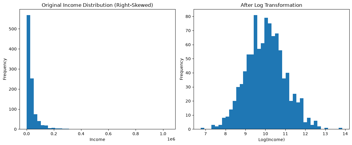
Remember, Log transformation is especially useful when a feature has a right-skewed distribution, meaning a small number of observations have extremely large values.

2c. Feature Encoding (Categorical Variables)

Machine learning models require numerical input, so categorical variables must be converted into numbers before they can be used in most algorithms. Example categorical feature:

Color
Red
Blue
Green

Several encoding techniques can be used depending on the type of categorical data and the number of categories.

(I) One-Hot Encoding

One-hot encoding creates a binary column for each category.

Color	Red	Blue	Green
Red	1	0	0
Blue	0	1	0

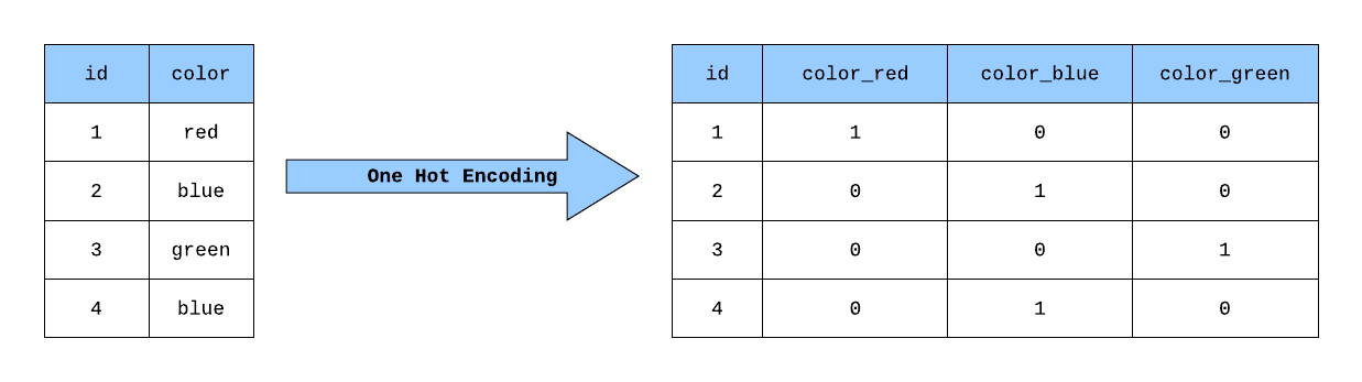Figure: One-Hot Encoding. Source: Medium

Suitable for: Nominal data (categories with no natural order)

Example code:

pd.get_dummies(df["color"])

(II) Label Encoding

Each category is assigned a numeric label.

Category	Encoded Value
Low	1
Medium	2
High	3

Figure: Label Encoding. Source: Daily Dose of Data Science

Suitable for: Ordinal data (categories with natural order)

Example code:

from sklearn.preprocessing import LabelEncoder

encoder = LabelEncoder()
df["category_encoded"] = encoder.fit_transform(df["category"])

Note: Label encoding may introduce artificial ordering when categories do not have a natural order.

(III) Frequency Encoding

Frequency encoding replaces categories with the frequency of their occurrence in the dataset.

Example:

Category	Frequency
A	0.40
B	0.35
C	0.25

Suitable for: High-cardinality categorical variables.

High-cardinality categorical variables are categorical features that contain a large number of unique categories (for example, hundreds or thousands of values such as city names, product IDs, or user IDs).

Example:

City
New York
Chicago
Los Angeles
Houston
Phoenix
…

If a feature contains many unique categories, using One-Hot Encoding would create a large number of new columns. In such cases, frequency encoding is often a more efficient approach.

Example Python Code:

freq = df["category"].value_counts(normalize=True)
df["category_freq"] = df["category"].map(freq)

(IV) Target (Mean) Encoding

Target encoding replaces each category with the average value of the target variable for that category.

Example:

City	Average House Price
City A	350000
City B	420000

In this approach, each category is replaced by the mean value of the target variable for that category.

For example, if houses in City A have an average price of 350,000, then all instances of City A may be encoded as 350000.

Suitable for: Categorical variables with many categories where the category has a relationship with the target variable.

Warning: Target encoding must be applied carefully to avoid data leakage, especially when the target values from the test data influence the encoding.

---

---

BONUS: What is Data Leakage?

Data leakage occurs when a model accidentally uses information that would not be available at prediction time. This can cause the model to appear very accurate during training, but perform poorly on new data.

Example of Leakage with Target Encoding

Suppose we want to predict house prices using the city as a feature.

City	Price
A	300000
A	400000
B	420000

If we compute the average price using the entire dataset, including the test data, the model indirectly gains information about the values it is supposed to predict. This creates data leakage.

Correct Approach

To avoid leakage:

1. Split the dataset into training and test sets first.

2. Compute the target encoding using only the training data.

3. Apply the learned encoding to the test data.

---

---

Example Python Code

import pandas as pd

# Example dataset
df = pd.DataFrame({
    "city": ["A", "A", "B", "B", "B"],
    "price": [300000, 400000, 420000, 410000, 430000]
})

# Compute mean target value for each category
target_mean = df.groupby("city")["price"].mean()

# Map the mean values back to the dataset
df["city_target_encoded"] = df["city"].map(target_mean)

df

Note: In practice, target encoding should be computed using training data only

(V) Probability Encoding

Probability encoding replaces categories with the conditional probability of the target variable given the category.

Example:

Category	P(Target = 1 | Category)
A	0.70
B	0.45

In this case, category A has a 70% probability of belonging to the target class, while category B has a 45% probability.

This approach is useful in classification problems where categories have different probabilities of belonging to the target class.

2d. Discretization (Binning)

Discretization, also called binning, is the process of converting continuous numerical variables into categorical groups (bins). Instead of using the exact numeric value, the variable is grouped into ranges.

This can help:

• simplify patterns in the data

• reduce noise

• improve interpretability

• make some models easier to train

Example

Age	Age_Group
22	Young
35	Adult
65	Senior

Instead of using exact ages, we categorize them into meaningful groups.

---

Example Code

import pandas as pd

df = pd.DataFrame({
    "age":[22,35,65,18,45]
})

df["age_group"] = pd.cut(df["age"], bins=[0,18,35,60,100])

df

Types of Binning:

• Equal Width Binning: Each bin has the same numerical range. Example:

  • 0–20

  • 20–40

  • 40–60

  • 60–80

• Equal Frequency Binning: Each bin contains approximately the same number of observations.

Example Python code:

df["age_bin"] = pd.qcut(df["age"], q=3)

Binning is helpful when:

• the exact numeric value is not necessary

• the variable has high variability

• interpretability is important

Example:

• Age → Age group

• Income → Income bracket

• Temperature → Cold / Moderate / Hot