20.5 Text Representation and Feature Extraction/Representation (Turning texts into vectors)

Machines cannot directly understand raw text; it must first be transformed into a numerical format. Feature extraction is the process of converting text into numerical representations—such as vectors capturing word frequencies or semantic meanings—so that machine learning models can interpret and use them for tasks such as sentiment analysis, classification, or translation.

There are several common approaches to representing text numerically:

20.5.1 Bag-of-Words (BoW)

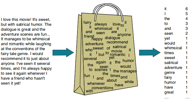
The Bag-of-Words (BoW) model is one of the simplest and most widely used text representation techniques. It represents text by counting the occurrences of each word in the document, completely ignoring grammar, word order, and context.

Concept: Treats each document as a “bag” of words—only the words themselves and their counts matter, not the order in which they appear.

Steps to follow:

• Tokenize the text (split into words).

• Build a vocabulary of all unique words across the corpus.

• Count the frequency of each word in each document.

  • Why? Each document is transformed into a vector where each position corresponds to a word in the vocabulary and the value is the frequency (count) of that word in the document.

Example:

Document: “Hi. This is an example sentence in an Example Document.”

• Tokenization (lowercased, punctuation removed):

• [hi, this, is, an, example, sentence, in, an, example, document]

• Vocabulary: [hi, this, is, an, example, sentence, in, document]

• Word Frequencies in the document: [1, 1, 1, 2, 2, 1, 1, 1]

• Word Frequencies in the document: [1, 1, 1, 2, 2, 1, 1, 1]→ corresponds to the order of the vocabulary.

So the BoW vector for this document is: [1, 1, 1, 2, 2, 1, 1, 1]

More Example(s):

Advantages: Simple and fast, works well for basic text classification.

Limitations: Ignores meaning and word order, produces sparse vectors with many zeros for large vocabularies. As vocabulary size can grow rapidly, increasing memory usage.

20.5.2 N-grams

BoW consider individual words (unigrams), but language meaning often depends on word combinations. N-grams are a variation of Bag of Words that captures sequences of N adjacent words.

Types:

• Unigram: single words (“machine”, “learning”)

• Bigram: pairs of words (“machine learning”)

• Trigram: triples (“natural language processing”)

Example:

N-grams help models understand phrases and partial word order, improving performance in many tasks. Still it has some limitation such as larger n can create exponentially larger vocabulary, rare phrases may not generalize well,etc.

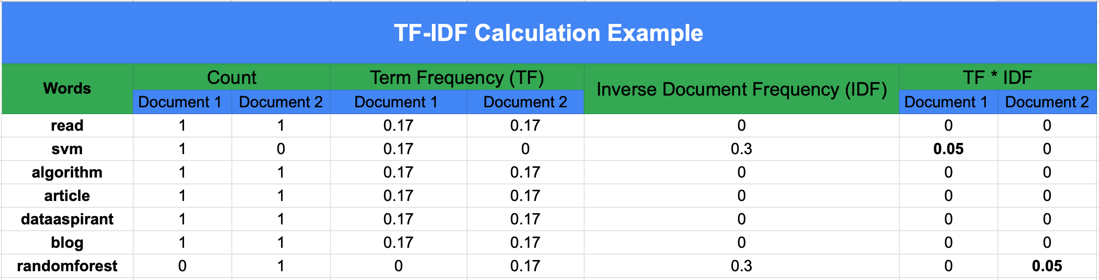
20.5.3 TF-IDF (Term Frequency-Inverse Document Frequency)

While BoW treats all words equally, TF-IDF weighs words based on how important they are to a document relative to a collection (corpus) of documents.

TF-IDF assigns more weight to informative words that are frequent in a specific document but rare across the corpus. This helps downweight common words like “the” or “is.”

Formula(s):

Term Frequency (TF): How often a word appears in a document.

\[ \mathrm{TF}(t, d) = \frac{\text{count}(t, d)}{\sum_{t' \in d} \text{count}(t', d)} \]

Document Frequency (DF): Number of documents that contain the term.

\[ \mathrm{DF}(t) = n_t \]

where (n_t) is the number of documents containing term (t).

Inverse Document Frequency (IDF): How rare a word is across all documents.

\[ \mathrm{IDF}(t) = \log\left(\frac{N}{\mathrm{DF}(t)}\right) \]

where (N) is the total number of documents.

TF–IDF:

\[ \mathrm{TF\text{-}IDF}(t, d) = \mathrm{TF}(t, d) \times \mathrm{IDF}(t) \]

Words that appear frequently in one document but rarely in others get higher weights, highlighting their importance. This helps reduce the impact of common words like “the” or “is” that appear everywhere.

Example: Calculating DF, IDF (base-10), TF, and TF–IDF

We have 3 documents:

1. machine learning is fun

2. machine learning is powerful

3. deep learning powers AI

Vocabulary:
$\( [\text{machine}, \text{learning}, \text{is}, \text{fun}, \text{powerful}, \text{deep}, \text{powers}, \text{ai}] \)$

---

Step 1 — Document Frequency (DF)

DF counts how many documents contain the term:

\[ DF(\text{machine}) = 2 \quad\text{(Doc1 & Doc2)} \]

\[ DF(\text{fun}) = 1 \quad\text{(Doc1 only)} \]

---

Step 2 — Inverse Document Frequency (IDF)

Using log base 10 (to match the numeric examples):

\[ IDF(t) = \log_{10}\!\left(\frac{N}{DF(t)}\right), \qquad N=3 \]

So:

\[ IDF(\text{machine}) = \log_{10}\!\left(\frac{3}{2}\right) \approx 0.17609 \]

\[ IDF(\text{fun}) = \log_{10}\!\left(\frac{3}{1}\right) \approx 0.47712 \]

(Interpretation: rarer terms → larger IDF.)

---

Step 3 — Term Frequency (TF)

For a term (t) in document (d):

\[ TF(t,d) = \frac{\text{count}(t,d)}{\text{total terms in } d} \]

Example for Doc 1 (“machine learning is fun”):

Total terms in Doc1 = 4.

\[ TF(\text{machine}, \text{Doc}_1) = \frac{1}{4} = 0.25 \]

\[ TF(\text{fun}, \text{Doc}_1) = \frac{1}{4} = 0.25 \]

---

Step 4 — TF–IDF

\[ TF\text{-}IDF(t,d) = TF(t,d)\times IDF(t) \]

For Doc 1:

\[ TF\text{-}IDF(\text{machine}, \text{Doc}_1) = 0.25 \times 0.17609 \approx 0.04402 \]

\[ TF\text{-}IDF(\text{fun}, \text{Doc}_1) = 0.25 \times 0.47712 \approx 0.11928 \]

(Despite equal TF in Doc1, “fun” scores higher because it is rarer across the corpus.)

Observation:
Even though “machine” and “fun” occur the same number of times in Doc 1, “fun” has a higher TF–IDF score because it is rarer in the overall corpus.

More Example(s):

20.5.4 Word Embeddings

Traditional frequency-based methods treat each word as independent, but words have semantic relationships. Word embeddings map words into dense vectors in a continuous space, where similar words lie close together.

Popular algorithms include: Word2Vec, GloVe

These embeddings capture relationships like: vector(“king”) – vector(“man”) + vector(“woman”) ≈ vector(“queen”)

20.5.5 Contextual Embeddings

Unlike static embeddings (Word2Vec, GloVe), contextual embeddings generate word representations based on surrounding words, capturing meaning that depends on context. For example, the word “bank” in “river bank” vs. “bank account” will have different embeddings.

Modern NLP models such as BERT and GPT produce contextual embeddings, enabling them to understand nuances and disambiguate meanings dynamically.