19.2 CNN Architecture Overview#
A typical CNN consists of the following layers:
Convolutional layer(s): Extracts features from the input dataset using learnable filters known as kernels applied to input images.
Pooling layer(s): Reduces the spatial dimensions of the input volume, speeding up computation, reducing memory usage, and helping prevent overfitting.
Fully connected layer(s): Used for the final classification or regression task.
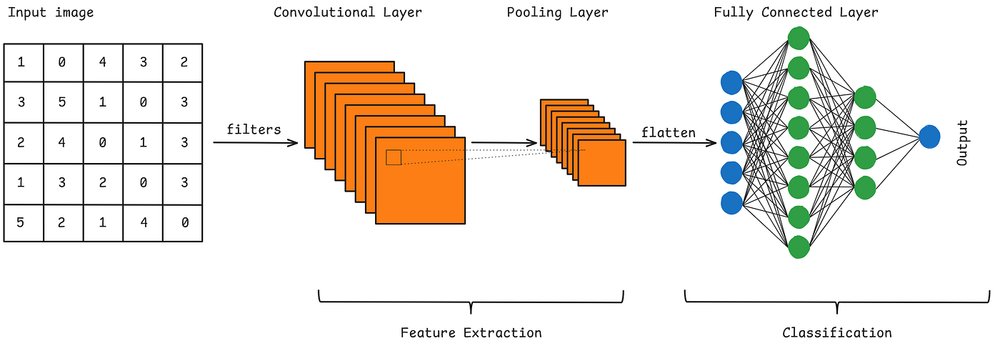
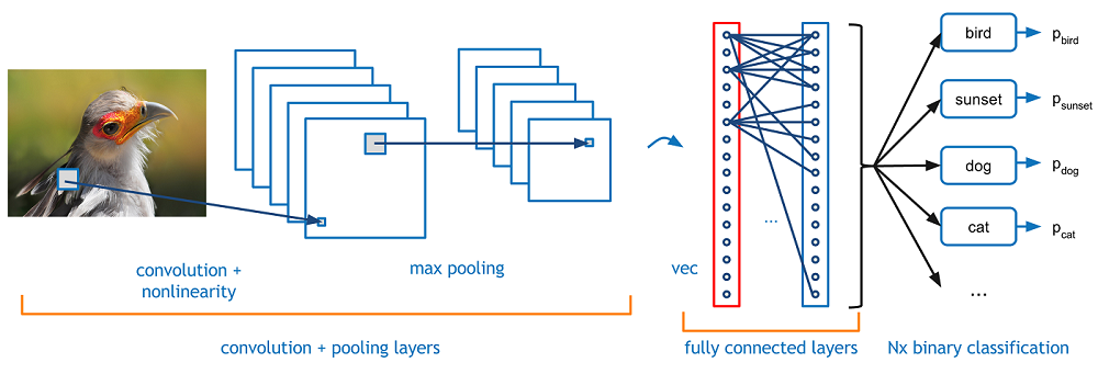
Figure: A simplified scheme of a simple CNN (with an example).
These layers are often supplemented with dropout and batch normalization for improved training stability.
19.2.1 Convolution Layer#
The convolutional layer is the core building block of a CNN. It applies a set of learnable filters (kernels) to the input, each detecting different features such as edges, textures, or patterns. A convolution operation refers to sliding a filter across the input image and computing the dot product between the filter weights and the corresponding input region. This operation produces a feature map (also known as activation map) that highlights where the detected feature appears in the input.
Figure: An example of a convolution operation applied to a 5×5 pixel, single-channel image using a 3×3 filter.
A Filter, or Kernel: in a CNN, is a small matrix used in the convolution operation. It’s a set of learnable weights that are applied to the input data to produce the output feature map. These small matrix of weights slides over the input data (such as an image), performs element-wise multiplication with the part of the input it is currently on, and then sums up all the results into a single output pixel. This process is known as convolution. Kernels are the key elements that allow CNNs to automatically learn spatial hierarchies of features within the input data. In image processing, a kernel might be a small matrix like 3x3 or 5x5.
Remember that, the filter values are trainable parameters, much like weights in a standard neural network. These values of the filters are learned during training through backpropagation, similar to weights in a traditional neural network. By sharing weights across the entire image, CNNs drastically reduce the number of parameters while retaining spatial information. The network learns multiple filters at each layer, each specialized to detect different features in the image, such as vertical edges, corners, or more complex textures.
There are some key parameters in a convolutional layer that include:
Kernel size (e.g., 3×3 or 5×5), which determines the receptive field.
Stride, the step size with which the filter moves across the image. A stride of 1 moves pixel-by-pixel, while a larger stride reduces spatial dimensions.
Padding, Controls whether we allow the output size to shrink or keep it the same as the input. It allows to adds extra pixels (usually zeros) around an image before convolution. It helps control the output size and preserves edge information.
Paddings are two types:
Same padding: Adds zeros so that the output has the same spatial dimensions (height and width) as the input. This helps preserve the size of the image throughout convolutional layers (same padding keeps the output the same size as the input, making it easier to stack many layers without losing resolution or cutting off edge information). Example: 5×5 input → 5×5 output (3×3 kernel, stride=1).
Valid padding: Adds no padding, so the convolution is only applied where the filter fully overlaps the input. This causes the output to shrink in size compared to the input. Example stride=1: 5×5 input → 3×3 output (3×3 kernel).
Remember: Higher strides = faster dimension reduction = less computation but potentially losing information.
Feature Map Size Calculation:#
The output spatial size (height or width) of a feature map after a convolution or pooling operation is calculated using:
\( \text{Output Size} = \left\lfloor \frac{\text{Input Size} - \text{Kernel Size} + 2 \times \text{Padding}}{\text{Stride}} \right\rfloor + 1 \)
Where:
Input Size (N): Height or width of the input (e.g., 32 for 32×32 image).
Kernel Size (F): Size of the filter (e.g., 3 for a 3×3 kernel)
Padding (P): Number of zeros added around the input (e.g., padding is 0 in ‘valid’ padding, and typically 1 for ‘same’ padding with a 3×3 kernel).
Stride (S): Step size of the filter (e.g., 1 = move 1 pixel, 2 = skip every other pixel)
⌊ ⌋: Floor operation (rounds down to the nearest neighbour)
Example:
For an input of size 32, a kernel size of 5, stride = 1, and padding = 0:
\( \text{Output Size} = \left\lfloor \frac{32 - 5 + 2 \times 0}{1} \right\rfloor + 1 = \left\lfloor 27 \right\rfloor + 1 = 28 \)
Output feature map size: 28 × 28.
Some More Common Examples:
32×32 input, 3×3 kernel:
stride=1, padding=0 → 30×30 output
stride=1, padding=1 → 32×32 output (same padding)
stride=2, padding=0 → 15×15 output
stride=2, padding=1 → 16×16 output
224×224 input (common ImageNet size), 7×7 kernel:
stride=2, padding=3 → 112×112 output (Used in many CNN architectures)
Key Notes:
‘Same’ padding maintains size when stride=1
Stride>1 reduces dimensions (useful for downsampling)
Pooling layers use same calculation (typically stride=2)
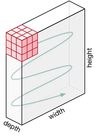
Movement of the Kernel:#
The kernel starts at the top-left corner of the input and moves right by the stride value, scanning horizontally. Once it reaches the edge, it returns to the left and shifts down by the stride to begin the next row. This top-to-bottom, left-to-right serpentine pattern continues until the entire input is covered.
 |
 |
| Kernel Movement (Static) | Kernel Movement (Animated) |
19.2.2 Activation Function (ReLU, Leaky ReLU, etc.)#
After each convolution, an activation function introduces non-linearity, allowing the network to learn complex patterns. The Rectified Linear Unit (ReLU) is the most widely used due to its simplicity and effectiveness in mitigating the vanishing gradient problem. ReLU outputs the input directly if it is positive; otherwise, it outputs zero.
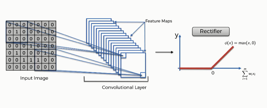 |
|
| Relu in CNN | How Relu Works |
The vanishing gradient problem occurs when gradients (used to update network weights during training) become very small, almost zero, especially in deep networks. This slows or stops learning because weights stop changing effectively. ReLU helps prevent this by allowing gradients to flow well for positive inputs.
In addition to introducing non-linearity, ReLU improves training efficiency by setting all negative values to zero. This creates sparsity in the network, meaning only the most important features (positive activations) are passed forward. This reduces complexity, helps the model focus on strong signals, and overall enables the CNN to learn faster and more effectively.
Other versions of ReLU, like Leaky ReLU and Parametric ReLU (PReLU), allow a small, non-zero output for negative input values instead of just zero. This helps avoid the problem of “dead neurons,” where some neurons stop learning completely.

19.2.3 Pooling Layers#
After applying convolution and activation (e.g., ReLU), a pooling layer (also called subsampling or downsampling) is used on the resulting feature map or activation map.
What is Pooling? A down-sampling operation that reduces the spatial dimensions (width and height) of the feature maps while keeping the most important information. This makes the network faster, uses less memory, and helps avoid overfitting.

Some of the most common types are:
Max Pooling: Selects the maximum value in each window of the feature map. It keeps the most important (strongest) features and helps detect edges or textures strongly.
Average Pooling: Computes the average of all values in each window, providing smoother downsampling. This leads to smoother results, but may lose some important details. It is less commonly used in modern CNNs than max pooling.
Sum Pooling: Adds up all the values in the window. It behaves similarly to average pooling, but keeps the total strength of the signa
Pooling helps in achieving translation invariance, meaning the network becomes less sensitive to the exact position of features in the input.
Note: Translation invariance is an important concept in computer vision that helps neural networks recognize objects even if they shift slightly in an image. This means the model becomes less sensitive to small movements or changes in position. For example, if a feature like a cat’s ear or an edge moves a little to the left or right, the network can still recognize it. This is made possible by pooling layers, which summarize small regions of the activation maps—using operations like max or average—rather than keeping exact pixel locations. This allows the network to focus more on what feature is present, rather than where exactly it is. As a result, even when the appearance of an object changes slightly or it appears in a different location, the model can still identify it accurately. This makes translation invariance especially valuable for tasks like object detection and image classification.
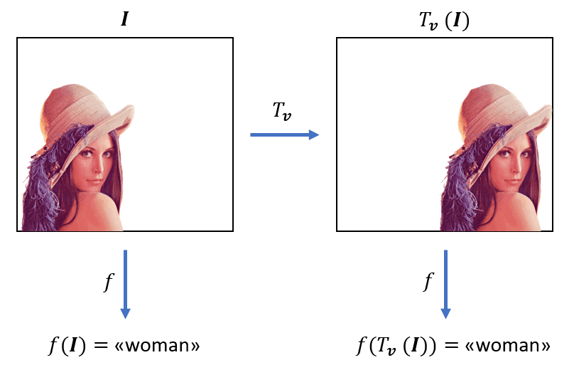
Figure: Let’s consider the images above. We can recognize a woman in both images even though the pixel values were shifted. An image classifier should predict the label “woman” for both images. In fact, the classifier output should not be influenced by the position of the target. Hence, the output of the classifier function is translation invariant. Ref:https://www.baeldung.com/cs/translation-invariance-equivariance.
19.2.4 Flattening and Fully Connected (Dense) Layer#
After several convolutional and pooling layers, the high-level features are flattened into a 1D vector and passed through one or more fully connected (dense) layers, just like in a traditional neural network. These layers perform the final classification or regression by combining all learned high-level features extracted by the convolutional layers. The last layer typically uses a softmax activation for classification or a linear activation for regression.
After several convolutional and pooling layers have extracted useful features, the output is flattened into a 1D vector—turning the multi-dimensional data into a simple list of numbers.
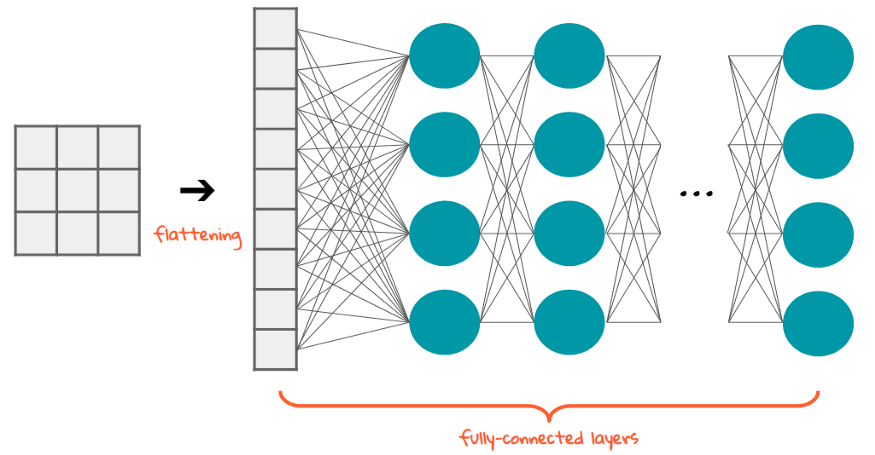 |
 |
| Flattening | Flattening in CNN |
This vector is then passed to one or more fully connected (dense) layers, just like in a traditional neural network. These layers connect every input to every output, allowing the model to learn complex patterns by combining all the features. In the final layer:
Classification tasks often use: Softmax activation for multi-class output Sigmoid for binary output.
Regression tasks usually use: Linear activation to produce continuous values.

This part of the network is responsible for making the final prediction based on the high-level features extracted earlier.