How the Regression Model Learns

How the Regression Model Learns#

The key idea behind regression is to find parameters (like $m$ and $b$) that minimize prediction error.

Residuals, Loss, and Cost Function#

To formalize the idea of “best fit,” we need a way to measure error.

Residual (Error)#

The residual represents how far off our prediction is from the true value (Difference between actual and predicted values). $$\text{error} = y - \hat{y}$$

$y$ → actual value
$\hat{y}$ → predicted value

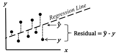
Residuals as Vertical Errors

Residual Distribution Around the Line

Left: Residuals shown as vertical distances between actual data points and the regression line. Right: Residuals ideally scattered randomly around zero, indicating a good model fit. Sources: StatisticsFromAtoZ.com | Statology.org

From the above visualization, you can see that, a residual can be visualized as the vertical distance between:

the actual data point
the regression line

The goal of regression is to make these vertical distances as small as possible. Here:

Positive residual → prediction is too low
Negative residual → prediction is too high

Loss Function (per data point)#

\[Loss = (y - \hat{y})^2\]

The loss function measures how wrong a single prediction is.

Cost Function (overall)#

\[MSE = \frac{1}{n} \sum (y - \hat{y})^2\]

Why squared error?

Avoid negative values
Penalize large errors more
Smooth optimization

Cost Function (Overall Error)#

\[MSE = \frac{1}{n} \sum (y - \hat{y})^2\]

The cost function aggregates error across all data points.

Provides a single number representing model performance
This is what we minimize during training

Important Distinction#

Residual → error for one data point
Loss → squared error for one data point
Cost → average loss across all data points

Understanding this hierarchy is critical for grasping how regression models are trained.

Error Measurement#

For each data point:

\[\text{error} = y_i - \hat{y}_i\]

To combine all errors, we use Mean Squared Error (MSE):

\[MSE = \frac{1}{n} \sum (y_i - \hat{y}_i)^2\]

Why square the error?

Ensures all values are positive
Penalizes larger errors more heavily

import matplotlib.pyplot as plt
from sklearn.linear_model import LinearRegression
import numpy as np

# sample data
X = np.array([[1], [2], [3], [4], [5]])
y = np.array([2, 4, 5, 4, 5])

model = LinearRegression()
model.fit(X, y)

y_pred = model.predict(X)

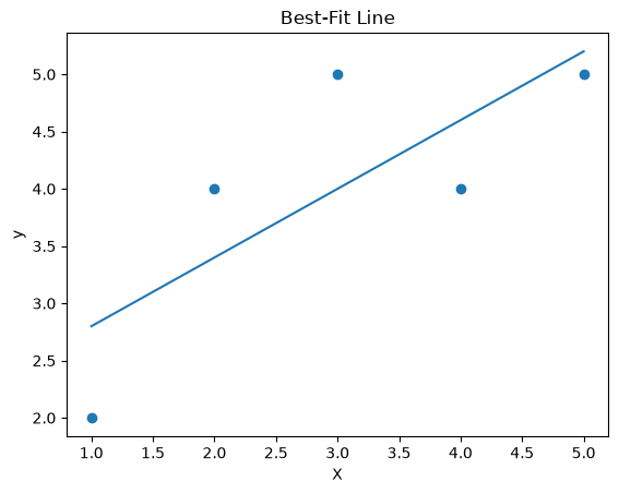
plt.scatter(X, y)
plt.plot(X, y_pred)
plt.title("Best-Fit Line")
plt.xlabel("X")
plt.ylabel("y")
plt.show()


'''
notice: how the line approximates data
that not all points lie on the line

'''

# Residual Visualization
plt.scatter(X, y)

# regression line
plt.plot(X, y_pred)

# draw residuals
for i in range(len(X)):
    plt.plot([X[i], X[i]], [y[i], y_pred[i]])

plt.title("Residuals (Errors)")
plt.show()

errors = y - y_pred
squared_errors = errors**2

print("Residuals:", errors)
print("Squared Errors:", squared_errors)
print("MSE:", np.mean(squared_errors))

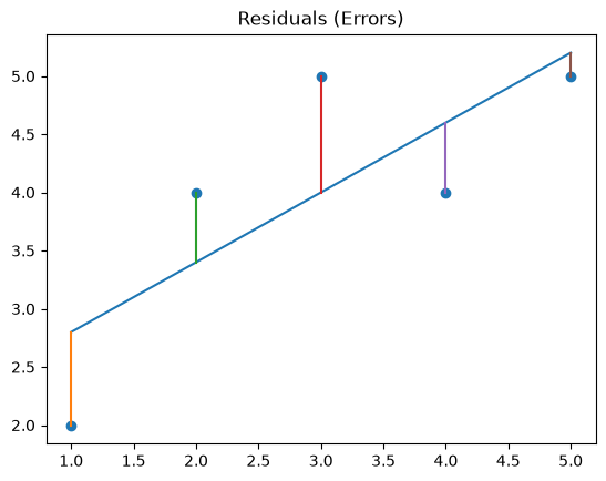
../_images/b0b105bae89a52d0be6997ac224154399cee0b92f1ed24ab7b2ff13c691b5826.png

../_images/e1c49d83028ec61ead8b2e7bb35350e69f3de3d885323be17022b33a62f5dd03.png

Residuals: [-0.8  0.6  1.  -0.6 -0.2]
Squared Errors: [0.64 0.36 1.   0.36 0.04]
MSE: 0.47999999999999987

At this stage, regression becomes more than just drawing a line.

It becomes an optimization problem:

Instead of manually choosing a line, we now aim to find the parameters of the model (e.g., slope and intercept) that minimize the overall prediction error.

In other words, we are solving:

Find the parameter values that minimize the cost function.

This shift from visualization to optimization is fundamental. It connects regression to a much broader class of machine learning algorithms, where learning is framed as minimizing a well-defined objective function.

Optimization in Linear Regression#

To minimize the cost function (typically Mean Squared Error), we use two main approaches:

The model adjusts parameters to minimize MSE using:

Gradient Descent (iterative approach)
Normal Equation (closed-form solution for linear regression)

Gradient Descent (Iterative Method)#

Starts with initial guesses for parameters
Updates parameters step-by-step
Moves in the direction that reduces error
Continues until convergence

Key idea: Move opposite to the gradient to reach the minimum.

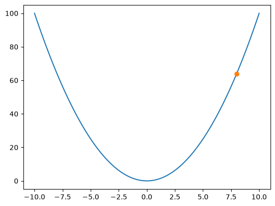
Gradient Descent Visualization#

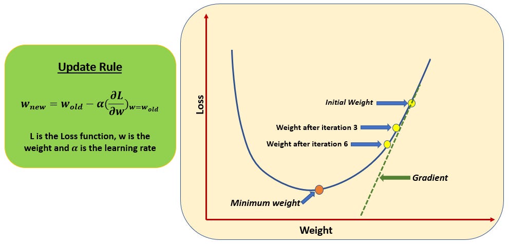
Gradient descent iteratively updates parameters by moving in the direction of steepest decrease in the cost function.

Gradient Descent: Pseudocode#

The following pseudocode describes how gradient descent iteratively updates model parameters to minimize the cost function.

General Gradient Descent Algorithm#

Input:

Training data $(X, y)$
Learning rate $\alpha$
Number of iterations (or convergence condition): $T$

Initialize:

Set initial values for parameters (e.g., slope $m$ and intercept $b$): $m = 0$, $b = 0$

Repeat until convergence: (For t = 1 to T:)

Compute predictions using current parameters
$\hat{y} = f(X)$
Compute the error (residuals)
$\text{error} = y - \hat{y}$
Compute gradients of the cost function with respect to parameters
- Gradient w.r.t slope
  $$dm = -\frac{2}{n} \sum X \cdot error$$
- Gradient w.r.t intercept
  $$db = -\frac{2}{n} \sum error$$

here: dm is gradient with respect to m and db is gradient with respect to b 4. Update parameters using the gradients

\[m = m - α * (\text{dm})\]

\[b = b - α * (\text{db})\]

Optionally compute cost (MSE) to monitor progress

Output:

Final optimized parameters (m, b): return final values of $m$ and $b$

At each step:

The gradient tells us which direction increases error
We move in the opposite direction to reduce error

** Stopping Criteria: **

The algorithm stops when:

Change in cost becomes very small, or
A fixed number of iterations is reached

Why Optimization Matters?#

This formulation allows us to:

Systematically improve predictions
Scale to complex models
Apply the same idea across many ML algorithms

Learning Rate ($\alpha$)#

A key component of gradient descent is the learning rate, usually denoted by $\alpha$.

The learning rate controls how large each update step is when adjusting the model parameters.

Why Learning Rate Matters#

At each step, gradient descent updates parameters as:

New parameter = Old parameter − $\alpha$ × (gradient)

The value of $\alpha$ determines how quickly (and how well) the model learns.

Effects of Different Learning Rates#

Too small ($\alpha$ is very low)
- Updates are tiny
- Convergence is very slow
- Training may take many iterations
Too large ($\alpha$ is very high)
- Steps may overshoot the minimum
- The model may oscillate or diverge
- May never converge
Well-chosen learning rate
- Efficient convergence
- Stable updates
- Faster training

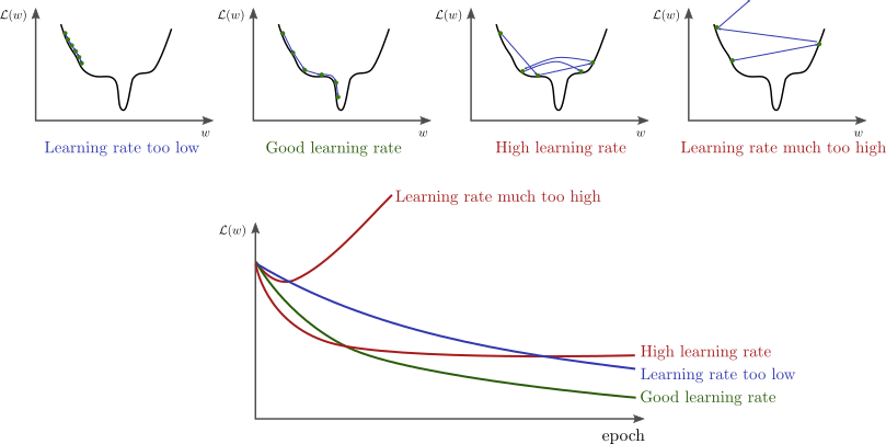
Different learning rates lead to very different behaviors: slow convergence, optimal convergence, or divergence.

Intuition#

You can think of gradient descent like walking downhill:

Learning rate = step size
Small steps → slow but safe
Large steps → fast but risky

The goal is to take steps that are large enough to move quickly, but small enough to avoid missing the minimum.

In practice, common learning rates include: 0.001, 0.01, 0.1, 0.05 etc. Often, the best value is found through experimentation or validation.

Summary:#

Gradient tells us which direction to move
Learning rate tells us how far to move

Both are essential for successfully minimizing the cost function.

import numpy as np
import matplotlib.pyplot as plt
from matplotlib.animation import FuncAnimation
from IPython.display import HTML

def f(x):
    return x**2

def grad(x):
    return 2*x

x = 8
learning_rate = 0.2
points = [x]

for _ in range(15):
    x = x - learning_rate * grad(x)
    points.append(x)

fig, ax = plt.subplots()
x_vals = np.linspace(-10, 10, 100)
ax.plot(x_vals, f(x_vals))
point, = ax.plot([], [], 'o')

def update(frame):
    x = points[frame]
    point.set_data([x], [f(x)])
    return point,

ani = FuncAnimation(fig, update, frames=len(points), interval=500)

HTML(ani.to_jshtml())

# Each step updates the model parameters to reduce error, gradually moving toward the minimum of the cost function.

../_images/e360e7b07e15bad6d4c1f00fdf0ab0ac775467f2b721ae41b75e649f3a10aa02.png

import numpy as np
import matplotlib.pyplot as plt
from matplotlib.animation import FuncAnimation
from IPython.display import HTML

# -----------------------------
# Sample data
# -----------------------------
X = np.array([1, 2, 3, 4, 5, 6], dtype=float)
y = np.array([2, 4, 5, 4, 5, 7], dtype=float)

# -----------------------------
# Gradient Descent settings
# -----------------------------
m = 0.0   # slope
b = 0.0   # intercept
lr = 0.05
epochs = 40

m_history = [m]
b_history = [b]

n = len(X)

# Run gradient descent and store parameters
for _ in range(epochs):
    y_pred = m * X + b

    dm = (-2/n) * np.sum(X * (y - y_pred))
    db = (-2/n) * np.sum(y - y_pred)

    m = m - lr * dm
    b = b - lr * db

    m_history.append(m)
    b_history.append(b)

# -----------------------------
# Animation
# -----------------------------
fig, ax = plt.subplots(figsize=(7, 5))
ax.scatter(X, y)
line, = ax.plot([], [], lw=2)

ax.set_xlim(X.min() - 0.5, X.max() + 0.5)
ax.set_ylim(y.min() - 1, y.max() + 1)
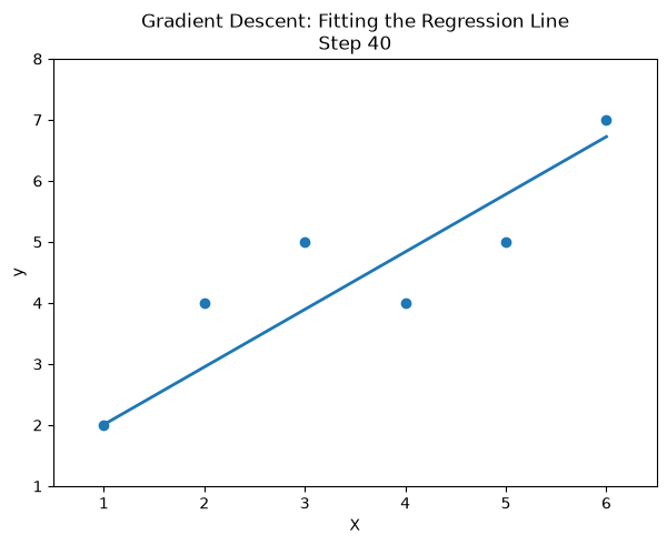
ax.set_title("Gradient Descent: Fitting the Regression Line")
ax.set_xlabel("X")
ax.set_ylabel("y")

def update(frame):
    m = m_history[frame]
    b = b_history[frame]
    x_vals = np.array([X.min(), X.max()])
    y_vals = m * x_vals + b
    line.set_data(x_vals, y_vals)
    ax.set_title(f"Gradient Descent: Fitting the Regression Line\nStep {frame}")
    return line,

ani = FuncAnimation(fig, update, frames=len(m_history), interval=300, blit=True)
HTML(ani.to_jshtml())

# This animation shows how gradient descent gradually updates the slope and intercept so that the regression line better fits the data over time.

../_images/9e95af98b5bef37d90ad5ab5d8bf0e723a1a0a8958b7c404f4347e0c2a57907c.png

# here is the learning rate comparison animation:

import numpy as np
import matplotlib.pyplot as plt
from matplotlib.animation import FuncAnimation
from IPython.display import HTML

def cost(x):
    return x**2

def grad(x):
    return 2 * x

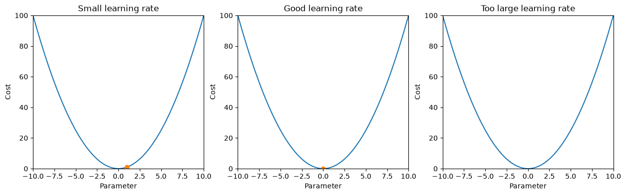
learning_rates = [0.05, 0.4, 1.1]
labels = ["Small learning rate", "Good learning rate", "Too large learning rate"]

steps_per_case = 20
all_points = []

for lr in learning_rates:
    x = 8.0
    points = [x]
    for _ in range(steps_per_case):
        x = x - lr * grad(x)
        points.append(x)
    all_points.append(points)

fig, axes = plt.subplots(1, 3, figsize=(15, 4))
x_vals = np.linspace(-10, 10, 400)

point_artists = []

for ax, label in zip(axes, labels):
    ax.plot(x_vals, cost(x_vals))
    ax.set_title(label)
    ax.set_xlabel("Parameter")
    ax.set_ylabel("Cost")
    ax.set_xlim(-10, 10)
    ax.set_ylim(0, 100)
    point, = ax.plot([], [], 'o')
    point_artists.append(point)

def update(frame):
    artists = []
    for i, point in enumerate(point_artists):
        x = all_points[i][frame]
        point.set_data([x], [cost(x)])
        artists.append(point)
    return artists

ani = FuncAnimation(fig, update, frames=steps_per_case + 1, interval=500, blit=True)
HTML(ani.to_jshtml())


'''
This comparison shows why the learning rate matters:
- A very small learning rate moves slowly and takes many steps.
- A well-chosen learning rate reaches the minimum efficiently.
- A very large learning rate overshoots and may fail to converge.
'''

'\nThis comparison shows why the learning rate matters:\n- A very small learning rate moves slowly and takes many steps.\n- A well-chosen learning rate reaches the minimum efficiently.\n- A very large learning rate overshoots and may fail to converge.\n'

../_images/537a2d55f5a6665d2cbd3d4a381c987aae1b68094e03e16c17a59429e133c380.png

Connecting Back to Regression#

In linear regression:

The parameters are slope ($m$) and intercept ($b$)
Gradient descent updates these parameters
Each update reduces prediction error

This is how the model “learns” from data.