import numpy as np
import matplotlib.pyplot as plt
from sklearn.cluster import KMeans
from sklearn.datasets import load_iris
from sklearn.preprocessing import StandardScaler

# Load and prepare data (from previous section)
iris = load_iris()
X = iris.data
scaler = StandardScaler()
X_scaled = scaler.fit_transform(X)
Here: Each color represents a different cluster The X markers represent the cluster centroids
Choosing the Right Value of K#
One practical challenge in K-Means is deciding:
How many clusters should we use?
The algorithm requires us to specify K in advance, but often we do not know the best value beforehand. A common way to choose K is the Elbow Method.
Elbow Method#
The Elbow Method helps us determine the optimal number of clusters (K) in K-Means. It examines how the inertia or WCSS changes as we increase the number of clusters. It works by:
Running K-Means for different values of K
Computing WCSS (inertia) for each K
Plotting K vs WCSS
As WCSS (inertia) measures how tightly the data points are grouped around their centroids, lower inertia means points are closer to their centroids.
As we increase K:
WCSS decreases (clusters become tighter)
But the improvement slows down after a point (becomes small).
We look for the point where the curve starts to bend like an elbow.
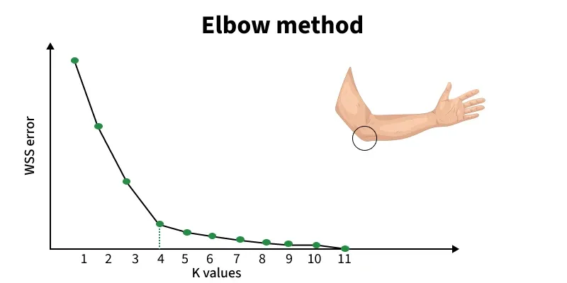
Figure: Elbow method showing WCSS (inertia) vs number of clusters (K). The “elbow point” indicates the optimal number of clusters. Source: GeeksforGeeks
The point where the curve bends is called the “elbow”. This is typically the best choice for K. From the above figure, notice how the curve drops sharply at first, then flattens; the curve bends sharply at K = 4, then 4 may be a reasonable number of clusters. this change in slope is the “elbow.”
# Step 1: Compute inertia for different values of K
inertia = []
for k in range(1, 10):
km = KMeans(n_clusters=k, random_state=42)
km.fit(X_scaled)
inertia.append(km.inertia_)
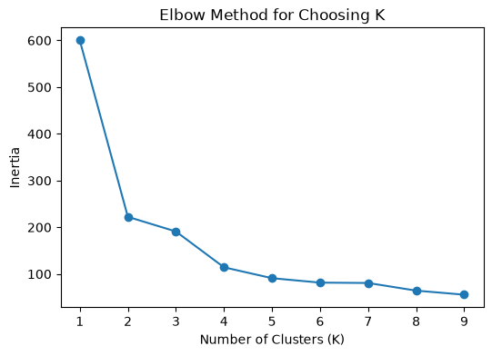
# Step 2: Plot the Elbow Curve
plt.figure(figsize=(6, 4))
plt.plot(range(1, 10), inertia, marker='o')
plt.xlabel("Number of Clusters (K)")
plt.ylabel("Inertia")
plt.title("Elbow Method for Choosing K")
plt.show()
Bonus Section: Silhouette Score (Evaluating Clustering Quality)#
While the Elbow Method helps us choose the number of clusters using WCSS, it does not always give a clear answer. To further evaluate clustering quality, we use: Silhouette Score
What is Silhouette Score?#
Silhouette Score measures how well each data point fits within its assigned cluster compared to other clusters.
For each point, it considers:
a(i) = average distance to points in the same cluster (intra-cluster distance)
b(i) = average distance to points in the nearest neighboring cluster (inter-cluster distance)
Interpretation: The score ranges from -1 to 1:
Close to +1 → well-clustered (far from other clusters)
Close to 0 → overlapping clusters
Close to -1 → wrongly assigned cluster
The intuition is that, a good clustering should have:
Small intra-cluster distance (points close together)
Large inter-cluster distance (clusters far apart)
Silhouette score combines both ideas into a single metric.
Using Silhouette Score to Choose K#
Instead of only relying on the Elbow Method, we can:
Compute silhouette score for different values of K
Choose the K with the highest silhouette score
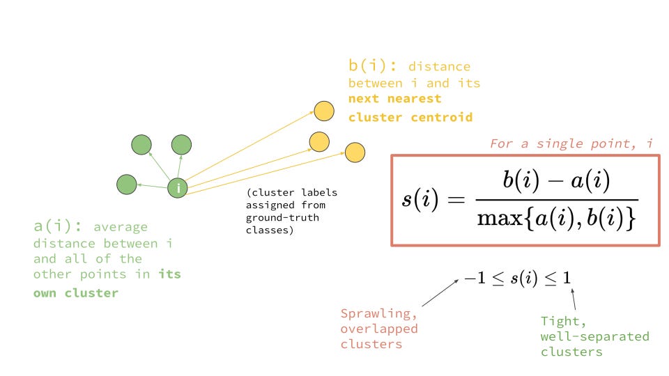
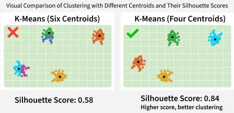
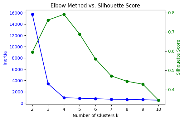
Figure: (a) Illustrating intra-cluster compactness and inter-cluster separation, (b) clustering of data points into groups based on similarity, (c) Elbow method and Silhouette score used to evaluate clustering quality. Sources: Medium; GeeksforGeeks
Python Example#
from sklearn.metrics import silhouette_score

scores = []

for k in range(2, 10):
    km = KMeans(n_clusters=k, random_state=42)
    labels = km.fit_predict(X_scaled)
    score = silhouette_score(X_scaled, labels)
    scores.append(score)

plt.plot(range(2, 10), scores, marker='o')
plt.xlabel("K")
plt.ylabel("Silhouette Score")
plt.title("Silhouette Score vs Number of Clusters")
plt.show()
Summary of K-Means#
K-Means is simple and powerful, but it comes with some assumptions:
Strengths:
Easy to understand and implement
Works well when clusters are compact and roughly spherical
Fast for large datasets
Limitation:s
Must choose K in advance
Sensitive to initialization
Can struggle when clusters have irregular shapes
Distance-based, so scaling matters