From Centrality to Community Detection

From Centrality to Community Detection#

In the previous section, we explored centrality measures to understand node importance in a graph. Where we learnt:

Degree centrality tells us which nodes have many direct connections. These nodes are locally important because they interact with many neighbors.
Closeness centrality captures how efficiently a node can reach all other nodes. Nodes with high closeness can spread information quickly across the network.
Betweenness centrality measures how often a node lies on shortest paths between other nodes. These nodes often act as bridges connecting different parts of the graph.

Transition: From Important Nodes to Important Edges#

So far, we focused on important nodes. Now, we shift our focus slightly:

Instead of asking “Which nodes are important?”, we ask:
“Which connections (edges) are critical for holding the network together?”

This is where the idea of betweenness becomes especially powerful.

Nodes with high betweenness sit between groups. Similarly, edges with high betweenness connect different communities.

Community Detection#

Real-world graphs are rarely random; nodes cluster into communities: groups with dense internal connections and sparse external ones.

Finding these communities reveals friend circles in social networks, topic clusters in citation graphs, functional modules in protein interaction networks, and fraud rings in financial graphs.

What is a “Community”?#

In many real-world networks, nodes naturally organize into groups, called communities.

Informally: a set of nodes that are more connected to each other than to the rest of the graph.

A community is a set of nodes that:

are densely connected to each other
have fewer connections to nodes outside the group

Think of friend circles in a social network or research groups in collaboration networks; within a community, there are many internal connections, while only a few edges connect it to other communities.

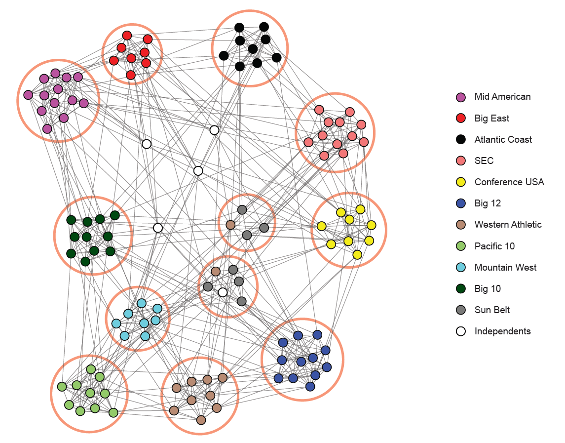
Community structure in an NCAA football network (teams grouped by conferences). Source: Stanford Network Analysis Project (SNAP)

Why Do Communities Form?#

Communities arise because:

People interact more within their group
Systems are organized into functional units
Networks evolve with localized connections

The ability to identify these communities through a process called community detection is arguably the most important and practical application of computer algorithms and graph theory.

Role of Connections Between Communities#

While communities are densely connected internally, they are typically linked to other groups by only a small number of edges. These edges act as bridges, enabling communication across different parts of the network.

From our earlier discussion on centrality:

Degree captures local connectivity
Closeness reflects how efficiently a node reaches others
Betweenness identifies nodes or edges that lie on many shortest paths

Key Insight: Edges with high betweenness often connect different communities because many shortest paths must pass through them.

Why Betweenness Reveals Communities#

Consider a network with two tightly connected groups and only a few connections between them. These cross-group edges:

appear frequently in shortest paths
carry a large portion of network flow
function as bridges between communities

If we remove these high-betweenness edges, the network naturally separates into distinct clusters.

Bridge Edge Example:#

A small number of edges connect two dense groups (bridge edges)

Community Separation via Edge Removal:#

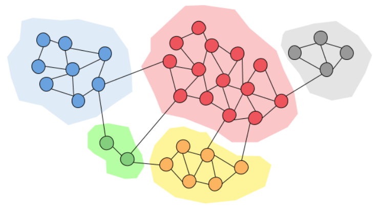
Removing high-betweenness edges gradually reveals community structure (Source: Miro Medium)

Interpretation:

Central edges → connect different groups; Removing them → graph splits into communitie.

We will deep-dive into the two foundational ideas: edge betweenness and the Girvan–Newman algorithm, and the quality metric modularity.

Edge Betweenness Centrality#

Edge betweenness measures how many shortest paths pass through a given edge:

\[C_B(e) = \sum_{s \neq t} \frac{\sigma_{st}(e)}{\sigma_{st}}\]

where $\sigma_{st}$ is the total number of shortest paths from $s$ to $t$, and $\sigma_{st}(e)$ is the number of those paths that use edge $e$.

Key intuition: edges that connect two otherwise loosely connected clusters will lie on a huge number of shortest paths. They are the bridges between communities. These edges will have very high betweenness scores.

Algorithm (Brandes):

For each source node $s$, run BFS/Dijkstra to find all shortest paths.
Back-propagate path counts along those trees to accumulate edge scores.
Repeat for all $n$ source nodes and sum.

Complexity: O(nm) for unweighted graphs (n nodes, m edges).

Note for This Course#

For simplicity, we will use the non-normalized version:

\[ C_B(e) = \sum_{s \neq t} \sigma_{st}(e) \]

Instead of dividing by $\sigma_{st}$, we simply count how many shortest paths pass through each edge.

Girvan–Newman Algorithm (Core Idea)#

The Girvan–Newman algorithm is based on a simple but powerful idea:

Repeatedly remove the most “important” edges to reveal hidden communities.

Proposed by Michelle Girvan and Mark Newman in 2002, this algorithm detects communities by progressively dismantling the graph; removing the edges that most bridge communities until the graph splits apart.

Algorithm steps:

Compute edge betweenness for every edge in the graph.
Identify the edge(s) with the highest betweenness score.
Remove that edge(s) from the graph
Recompute edge betweenness for all remaining edges (structure has changed) .
Repeat until the graph breaks into the desired number of components (or until all edges are gone).

As edges are removed, the graph gradually breaks into separate components, which correspond to communities.

Why does this work?

Edges that connect two communities tend to carry most of the shortest-path traffic between them, which gives them very high betweenness values.

In contrast, edges within a community are part of a dense structure, so there are many alternative paths and no single edge is as critical.

As a result, when we remove the edge with the highest betweenness, we are typically cutting a bridge between communities, allowing the graph to separate naturally into clusters.

Computing Edge Betweenness (Intuition)#

Edge betweenness answers the question:

Which edges are used the most when moving from one node to another?

Consider a graph that naturally splits into two groups. To travel from a node on one side to a node on the other, most shortest paths must pass through a small set of connecting edges.

Edges connecting two groups are used more frequently in shortest paths

For example, if node 1 wants to reach node 12, a shortest path might look like:

1 → 3 → 7 → 8 → 12

Here, the edge between nodes 7 and 8 lies on many such paths, making it highly important. Edges like this have high betweenness because they carry a large portion of the network’s shortest-path traffic.

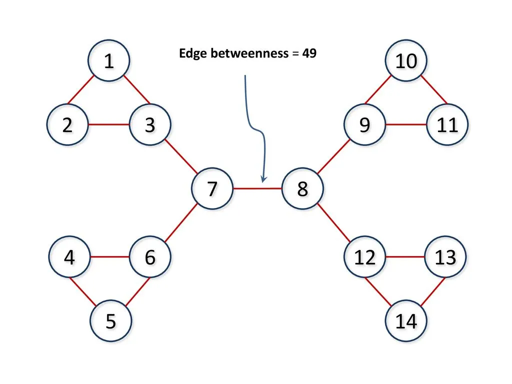
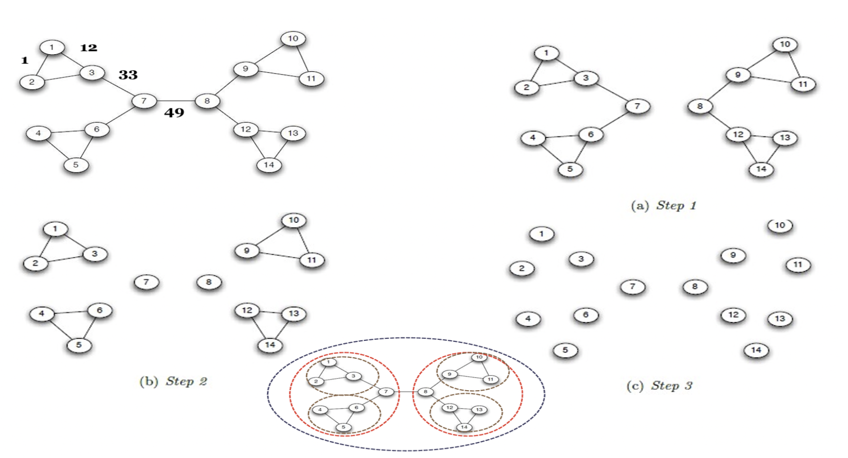
Why is Edge Betweenness of (7,8) = 49?#

The edge between nodes 7 and 8 connects two large parts of the graph (left and right). Any shortest path from a node on the left to a node on the right must pass through this edge.

Left side has 7 nodes: {1,2,3,4,5,6,7}
Right side has 7 nodes: {8,9,10,11,12,13,14}

The total number of shortest paths between the two sides is:

\[ 7 \times 7 = 49 \]

Each pair contributes one shortest path, and all of them pass through edge (7,8).

Key Insight:

The edge (7,8) has very high betweenness because:

it is the only bridge between the two halves
it carries all cross-group shortest paths

This is why it gets the highest score and is removed first in the Girvan–Newman algorithm.

To compute edge betweenness, we find shortest paths between all pairs of nodes (e.g., using BFS for unweighted graphs) and count how many times each edge is used. At the end, each edge has a score representing how often it is used.

The edge with the highest score (highest betweenness) is removed, and the process is repeated on the updated graph.

Note: If multiple edges have the same highest value, any one of them can be removed (or all of them together, depending on the implementation).

Complexity:

Each edge removal requires recomputing betweenness in O(nm) time, and repeating this many times leads to O(m² n) overall. Because of this, Girvan–Newman is slow for large graphs, but works well for small networks and for building intuition.

Output: The result of the algorithm is a dendrogram, a tree-like representation that shows how the graph splits over time.

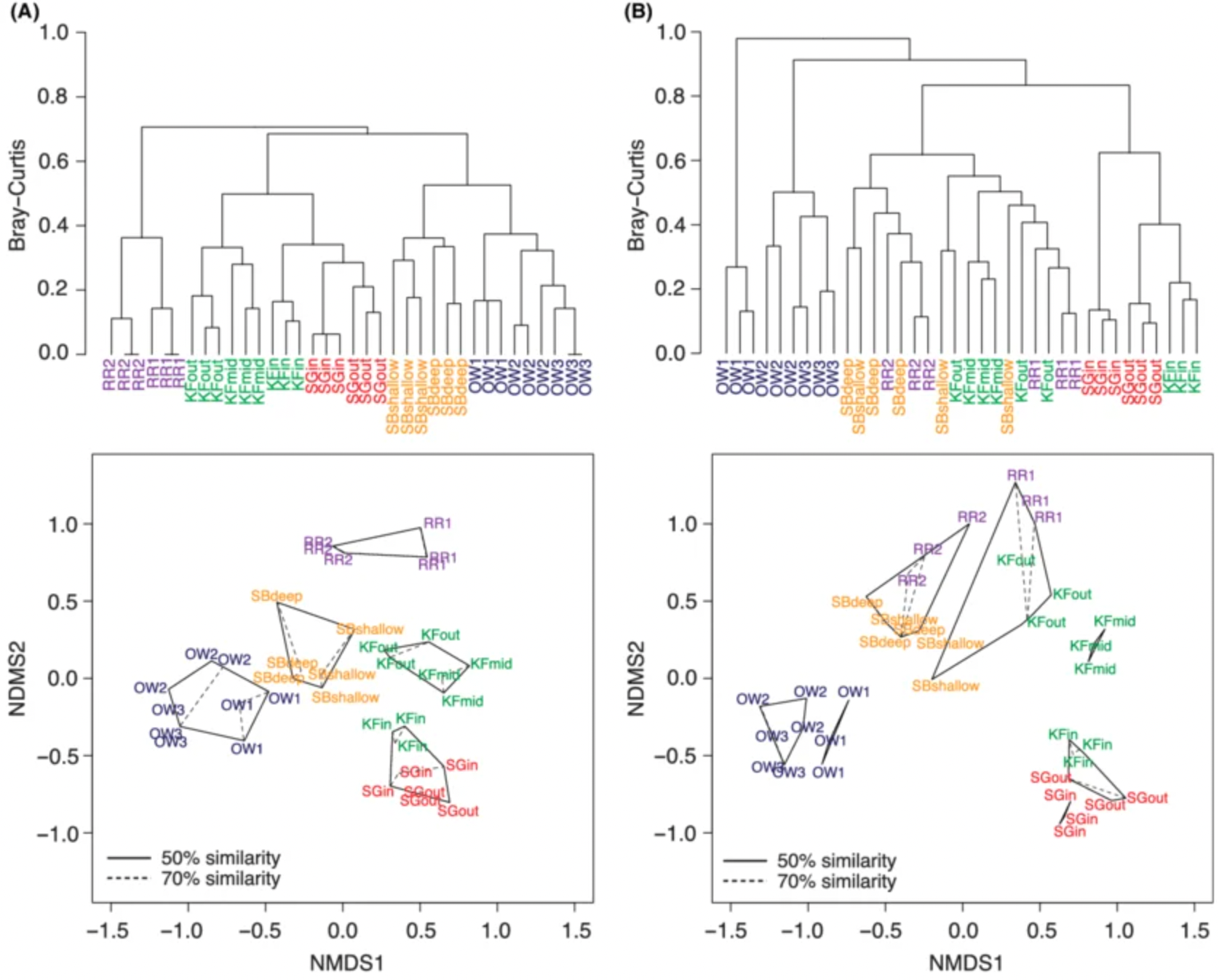
Example of a dendrogram showing hierarchical splitting of groups, Source: Jesse Port et al.,Hierarchical clustering of vertebrate communities

The algorithm starts with the whole graph and gradually splits it into smaller groups. By cutting the tree at different levels, we can obtain a few large communities or many smaller ones.

Selecting Number of Communities#

Wait! Girvan–Newman keeps removing edges. If we remove all edges, every node becomes its own community. So the key question is: when should we stop?

The graph starts as one group and gradually splits into smaller communities

One simple approach is to stop when we reach a desired number of groups. This works only if we already know how many communities we expect.

A more flexible approach is to use modularity. After each split, we measure how good the community partition is. The partition with the highest modularity is considered the best because it has many connections within communities and fewer connections between communities.

Modularity: Measuring Partition Quality#

Girvan–Newman tells us how to split a graph, but modularity helps decide which split is best. Modularity $Q$ measures the quality of a community partition.

\[ Q = \frac{1}{2m} \sum_{i,j} \left[ A_{ij} - \frac{k_i k_j}{2m} \right] \delta(c_i, c_j) \]

where:

$m$ = number of edges
$A_{ij}$ = 1 if edge $(i,j)$ exists, 0 otherwise
$k_i$ = degree of node $i$
$\frac{k_i k_j}{2m}$ = expected number of edges between $i$ and $j$ in a random graph
$\delta(c_i, c_j)$ = 1 if $i$ and $j$ are in the same community, 0 otherwise

Intuition#

Modularity compares the number of edges within communities to what we would expect by chance:

\[ Q \propto \sum_{\text{communities}} \left( \text{actual edges within group} - \text{expected edges within group} \right) \]

Higher $Q$ means stronger community structure (more internal connections than expected).

Interpretation#

Q value	Interpretation
< 0	Worse than random
0	No clear community structure
0.3 – 0.7	Meaningful community structure
> 0.7	Very strong community structure (rare)

Stop criterion (Girvan–Newman): compute $Q$ after each split and choose the partition with the highest value.

Small Modularity Calculation Example#

Consider this graph: A — B C — D

Edges: (A–B), (C–D)

So:

Number of edges: $m = 2$
Communities:
- Community 1: {A, B}
- Community 2: {C, D}

We use:

\[ Q = \frac{1}{2m} \sum_{i,j} \left[ A_{ij} - \frac{k_i k_j}{2m} \right] \delta(c_i, c_j) \]

Step 1: Node Degrees#

$k_A = 1$, $k_B = 1$, $k_C = 1$, $k_D = 1$

Step 2: Compute for pairs in same community#

Community 1: (A, B)#

$A_{AB} = 1$
Expected: $\frac{k_A k_B}{2m} = \frac{1 \cdot 1}{4} = 0.25$

Contribution: $$ 1 - 0.25 = 0.75 $$

Community 2: (C, D)#

Same: $$ 1 - 0.25 = 0.75 $$

Step 3: Final Q#

Sum = $0.75 + 0.75 = 1.5$

\[ Q = \frac{1}{2m} \times 1.5 = \frac{1}{4} \times 1.5 = 0.375 \]

$Q = 0.375$ indicates a meaningful community structure
(since internal edges are higher than expected by chance)

Summary of the Chapter#

Concept	Key idea
Graph G = (V, E)	Nodes + edges encode entities and relationships
3 representations	Matrix (fast lookup), List (memory efficient), Dictionary (flexible, weighted)
Featurization	Convert structure into numeric vectors for ML
Degree centrality	Who has the most direct connections?
Closeness centrality	Who spreads information fastest?
Betweenness centrality	Who is the gatekeeper / bridge?
Community	Groups of nodes densely connected internally
Girvan–Newman	Detect communities by removing high-betweenness edges
Modularity (Q)	Measures how strong a community partition is
BFS	Level-by-level traversal; shortest paths in unweighted graphs
DFS	Deep-first traversal; cycle detection, topological sort
PageRank	Importance via incoming link quality — powers Google Search

The same mathematical object; a graph; routes your commute, serves your Netflix recommendations, and helps researchers discover new medicines. The abstraction is the power.

BONUS: Graph Processing#

Graph processing means running algorithms over the graph structure to extract insights or support decisions.

Core processing tasks#

Task	Goal	Algorithm	Use case
Traversal	Visit all reachable nodes	BFS, DFS	Component finding, web crawling
Shortest path	Minimum hops or cost	Dijkstra, A*, BFS	Navigation, network routing
Minimum spanning tree	Connect all nodes at minimum cost	Kruskal, Prim	Laying cables, circuit design
Community detection	Find dense subgroups	Louvain, Label Propagation	Social clusters, fraud rings
Node ranking	Score nodes by importance	PageRank, HITS	Web search, citation analysis
Link prediction	Predict missing edges	Common neighbors, GNN	Friend suggestions
Graph classification	Label an entire graph	GCN, GraphSAGE	Molecule toxicity, code analysis

BONUS: Graph neural networks (GNNs)#

Classical graph algorithms are hand-crafted rules. Graph Neural Networks learn representations directly from graph structure and node/edge features, enabling tasks like:

Node classification: predict a node’s category (is this account a bot?)
Link prediction: will these two nodes form an edge? (friend suggestion, drug-target interaction)
Graph classification: classify an entire graph (is this molecule toxic?)

Traditional ML → manual feature engineering

Graph Neural Networks → automatic feature learning
Key Idea: Feature(node) = function(node + neighbors)

The core operation is message passing: each node aggregates feature vectors from its neighbors, transforms them, and updates its own representation. After k rounds, a node’s embedding captures its k-hop neighborhood. This is the basis of models like GCN, GAT, and GraphSAGE, which power modern recommendation systems at Pinterest, Uber, and Alibaba.

In this book, we are not going to cover GNN in details but here is an interesting article to read: https://distill.pub/2021/gnn-intro/.